Optimal rational approximation

A few days ago I wrote about the approximation

for cosine due to the Indian astronomer Aryabhata (476–550) and gave this plot of the error.

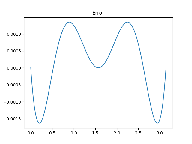I said that Aryabhata’s approximation is “not quite optimal since the ripples in the error function are not of equal height.” This was an allusion to the equioscillation theorem.

Chebyshev proved that an optimal polynomial approximation has an error function that has equally large positive and negative oscillations. Later this theorem was generalized to rational approximations through a sequence of results by de la Vallée Poussin, Walsh, and Achieser. Here’s the formal statement of the theorem from [1] in the context of real-valued rational approximations with numerators of degree m and denominators of degree n

Theorem 24.1. Equioscillation characterization of best approximants. A real function f in C[−1, 1] has a unique best approximation r*, and a function r is equal to r* if and only if f − r equioscillates between at least m + n + 2 − d extremes where d is the defect of r.

When the theorem says the error equioscillates, it means the error alternately takes on ± its maximum absolute value.

The defect is non-zero when both numerator and denominator have less than maximal degree, which doesn’t concern is here.

We want to find the optimal rational approximation for cosine over the interval [−π/2, π/2]. It doesn’t matter that the theorem is stated for continuous functions over [−1, 1] because we could just rescale cosine. We’re looking for approximations with (m, n) = (2, 2), i.e. ratios of quadratic polynomials, to see if we can improve on the approximation at the top of the post.

The equioscillation theorem says our error should oscillate at least 6 times, and so if we find an approximation whose error oscillates as required by the theorem, we know we’ve found the optimal approximation.

I first tried finding the optimal approximation using Mathematica’s MiniMaxApproximation function. But this function tries to optimize relative error and I’m trying to minimize absolute error. Minimizing relative error creates problems because cosine evaluates to zero at the ends of interval ±π/2. I tried several alternatives and eventually decided to take another approach.

Because the cosine function is even, the optimal approximation is even. Which means the optimal approximation has the form

(a + bx²) / (c + dx²)

and we can assume without loss of generality that a = 1. I then wrote some Python code to minimize the error as a function of the three remaining variables. The results were b = −4.00487004, c = 9.86024544, and d = 1.00198695, very close to Aryabhata’s approximation that corresponds to b = −4, c = π², and d = 1.

Here’s a plot of the error, the difference between cosine and the rational approximation.

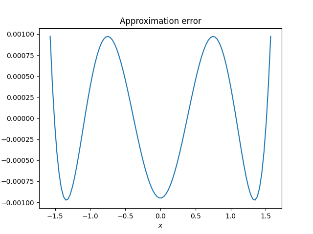
The absolute error takes on its maximum value seven times, alternating between positive and negative values, and so we know the approximation is optimal. However sketchy my approach to finding the optimal approximation may have been, the plot shows that the result is correct.

Aryabhata’s approximation had maximum error 0.00163176 and the optimal approximation has maximum error 0.00097466. We were able to shave about 1/3 off the maximum error, but at a cost of using coefficients that would be harder to use by hand. This wouldn’t matter to a modern computer, but it would matter a great deal to an ancient astronomer.

Related posts

• Economizing approximations
• Chebyshev approximation

[1] Approximation Theory and Approximation Practice by Lloyd N. Trefethen