 10 hours ago
3
10 hours ago
3
Club.noww.in
A complete guide on how to apply the Q-Learning method in Python to optimize inventory management and reduce costs
 Photo by Petrebels on Unsplash
Inventory Management — What Problem Are We Solving?
Imagine you are managing a bike shop. Every day, you need to decide how many bikes to order from your supplier. If you order too many, you incur high holding costs (cost of storing bikes overnight); if you order too few, you might miss out on potential sales. Here, the challenge is to develop a (ordering) strategy that balances these trade-offs optimally. Inventory management is crucial in various industries, where the goal is to determine the optimal quantity of products to order periodically to maximize profitability.
Why Reinforcement Learning for Inventory Management?
Previously, we discussed approaching this problem using Dynamic Programming (DP) with the Markov Decision Process (MDP) Here. However, the DP approach requires a complete model of the environment (in this case, we need to know the probability distribution of demand), which may not always be available or practical.
Here, the Reinforcement Learning (RL) approach is presented, which overcomes that challenge by following a “data-driven” approach.The goal is to build a “data-driven” agent that learns the best policy (how much to order) through interacting with the environment (uncertainty). The RL approach removes the need for prior knowledge about the model of the environment. This post explores the RL approach, specifically Q-learning, to find the optimal inventory policy.
How to Frame the Inventory Management Problem?
Before diving into the Q-learning method, it’s essential to understand the basics of the inventory management problem. At its core, inventory management is a sequential decision-making problem, where decisions made today affect the outcomes and choices available tomorrow. Let’s break down the key elements of this problem: the state, uncertainty, and recurring decisions.
State: What’s the Current Situation?
In the context of a bike shop, the state represents the current situation regarding inventory. It’s defined by two key components:
α (Alpha): The number of bikes you currently have in the store. (referred to as On-Hand Inventory)
β (Beta): The number of bikes that you ordered yesterday and are expected to arrive tomorrow morning (36 hours delivery lead time). These bikes are still in transit. (referred to as On-Order Inventory)
Together, (α,β) form the state, which gives a snapshot of your inventory status at any given moment.
Uncertainty: What Could Happen?
Uncertainty in this problem arises from the random demand for bikes each day. You don’t know exactly how many customers will walk in and request a bike, making it challenging to predict the exact demand.
Decisions: How Many Items Should you Order Every Day?
As the bike shop owner, you face a recurring decision every day: How many bikes should you order from the supplier? . Your decision needs to account for both the current state of your inventory (α,β) and also the uncertainty in customer demand for the following day.
A typical 24-hour cycle for managing your bike shop’s inventory is as follows:
6 PM: Observe the current state St:(α,β) of your inventory. (State)
6 PM: Make the decision on how many new bikes to order. (Decision)
6 AM: Receive the bikes you ordered 36 hours ago.
8 AM: Open the store to customers.
8 AM — 6 PM: Experience customer demand throughout the day. (Uncertainty)
6 PM: Close the store and prepare for the next cycle.
A graphical representation of the inventory management process is shown below:
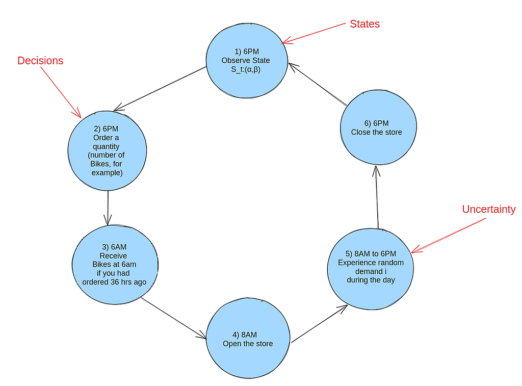 A typical 24-hour cycle for inventory management — image source: Author
What is Reinforcement Learning?
Reinforcement Learning (RL) is a data-driven method that focuses on learning how to make sequences of decisions (following a policy) to maximize a cumulative reward. It's similar to how humans and animals learn what action to take through trial and error. In the context of inventory management, RL can be used to learn the optimal ordering policy that minimizes the total cost of inventory management.
The key components of the RL approach are:
Agent: The decision-maker who interacts with the environment.
Environment: The external system with which the agent interacts. In this case, the environment is the random customer demand.
State: The current situation or snapshot of the environment.
Action: The decision or choice made by the agent.
Reward: The feedback signal that tells the agent how well it’s doing.
The goal of the agent (decision-maker) is to learn the optimal policy, which is a mapping from states to actions that maximize the cumulative reward over time.
In the context of inventory management, the policy tells the agent how many bikes to order each day based on the current inventory status and the uncertainty in customer demand.Implementing Reinforcement Learning for Inventory Optimization Problem
Q-learning is a model-free reinforcement learning algorithm that learns the optimal action-selection policy for any given state. Unlike the DP approach, which requires a complete model of the environment, Q-learning learns directly from the interaction with the environment (here, uncertainty and the reward it gets) by updating a Q-table.
The key components of Q-Learning
In our case, the agent is the decision-maker (the bike shop owner), and the environment is the demand from customers. The state is represented by the current inventory levels (alpha, beta), and the action is how many bikes to order. The reward is the cost associated with both holding inventory and missing out on sales. Q-Table is a table that stores the expected future rewards for each state-action pair.
Initialization of Q Table
In this work, the Q-table is initialized as a dictionary named Q. States are represented by tuples (alpha, beta), where: alpha is the number of items in stock (on-hand inventory). beta is the number of items on order (on-order inventory).
Actions are possible inventory order quantities that can be taken in each state. For each state (alpha, beta), the possible actions depend on how much space is left in the inventory (remaining capacity = Inventory Capacity — (alpha + beta)). The restriction is that the number of items ordered cannot exceed the remaining capacity of the inventory.
The schematic design of the Q value is visualized below:
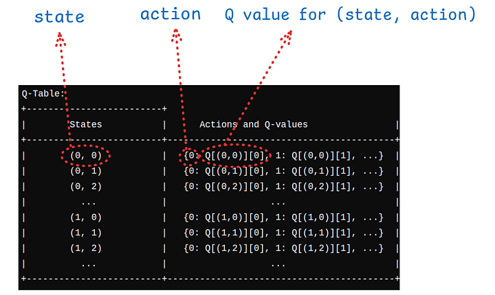 A schematic design of the Q dictionary is visualized — Image source: Author
The Q dictionary can be initialized as:
def initialize_Q(self):# Initialize the Q-table as a dictionary
Q = {}
for alpha in range(self.user_capacity + 1):
for beta in range(self.user_capacity + 1 - alpha):
state = (alpha, beta)
Q[state] = {}
max_action = self.user_capacity - (alpha + beta)
for action in range(max_action + 1):
Q[state][action] = np.random.uniform(0, 1) # Small random values
return Q
As the above code shows, Q-values (Q[state][action]) are initialized with small random values to encourage exploration.
The Q-Learning Algorithm
The Q-learning method updates a table of state-action pairs based on rewards from the environment (here, interacting with the environment comes). Here’s how the algorithm works in three steps:
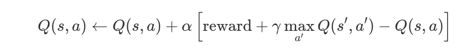 Q-Learning Equation — Image Source: Author
Where s is the current state, a is the action taken, s’ is the next state, ( α ) is the learning rate. and ( γ ) is the discount factor.
We breakdown the equation, and rewrote it in three parts down here:
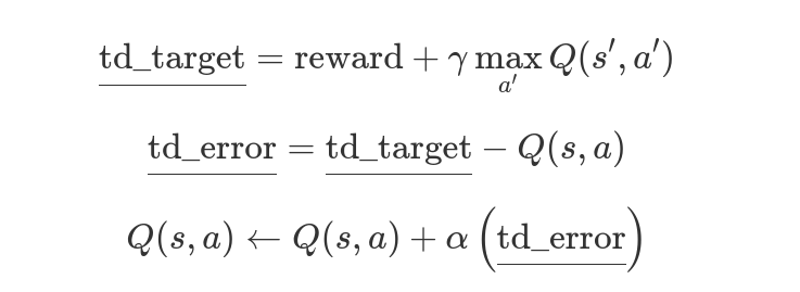 Q-Learning Equation — Image Source: Author
The translation of the above equations to Python code is as follows:
def update_Q(self, state, action, reward, next_state):# Update the Q-table based on the state, action, reward, and next state
best_next_action = max(self.Q[next_state], key=self.Q[next_state].get)
# reward + gamma * Q[next_state][best_next_action]
td_target = reward + self.gamma * self.Q[next_state][best_next_action]
# td_target - Q[state][action]
td_error = td_target - self.Q[state][action]
# Q[state][action] = Q[state][action] + alpha * td_error
self.Q[state][action] += self.alpha * td_error
At the above function, the equivalent equation of each line has been shown as a comment on top of each line.
Simulating Transitions and Rewards in Q-Learning for Inventory Optimization
The current state is represented by a tuple (alpha, beta), where: alpha is the current on-hand inventory (items in stock), beta is the current on-order inventory (items ordered but not yet received), init_inv calculates the total initial inventory by summing alpha and beta.
Then, we need to simulate customer demand using Poisson distribution with lambda value “self.poisson_lambda”. Here, the demand shows the randomness of customer demand:
alpha, beta = stateinit_inv = alpha + beta
demand = np.random.poisson(self.poisson_lambda)
Note: Poisson distribution is used to model the demand, which is a common choice for modeling random events like customer arrivals. However, we can either train the model with historical demand data or live interaction with environment in real time. In its core, reinforcement learning is about learning from the data, and it does not require prior knowledge of a model.
Now, the “next alpha” which is in-hand inventory can be written as max(0,init_inv-demand). What that means is that if demand is more than the initial inventory, then the new alpha would be zero, if not, init_inv-demand.
The cost comes in two parts. Holding cost: is calculated by multiplying the number of bikes in the store by the per-unit holding cost. Then, we have another cost, which is stockout cost. It is a cost that we need to pay for the cases of missed demand. These two parts form the “reward” which we try to maximize using reinforcement learning method.( a better way to put is we want to minimize the cost, so we maximize the reward).
new_alpha = max(0, init_inv - demand)holding_cost = -new_alpha * self.holding_cost
stockout_cost = 0
if demand > init_inv:
stockout_cost = -(demand - init_inv) * self.stockout_cost
reward = holding_cost + stockout_cost
next_state = (new_alpha, action)
Exploration — Exploitation in Q-Learning
Choosing action in the Q-learning method involves some degree of exploration to get an overview of the Q value for all the states in the Q table. To do that, at every action chosen, there is an epsilon chance that we take an exploration approach and “randomly” select an action, whereas, with a 1-ϵ chance, we take the best action possible from the Q table.
def choose_action(self, state):# Epsilon-greedy action selection
if np.random.rand() < self.epsilon:
return np.random.choice(self.user_capacity - (state[0] + state[1]) + 1)
else:
return max(self.Q[state], key=self.Q[state].get)
Training RL Agent
The training of the RL agent is done by the “train” function, and it is follow as: First, we need to initialize the Q (empty dictionary structure). Then, experiences are collected in each batch (self.batch.append((state, action, reward, next_state))), and the Q table is updated at the end of each batch (self.update_Q(self.batch)). The number of episodes is limited to “max_actions_per_episode” in each batch. The number of episodes is the number of times the agent interacts with the environment to learn the optimal policy.
Each episode starts with a randomly assigned state, and while the number of actions is lower than max_actions_per_episode, the collecting data for that batch continues.
def train(self):self.Q = self.initialize_Q() # Reinitialize Q-table for each training run
for episode in range(self.episodes):
alpha_0 = random.randint(0, self.user_capacity)
beta_0 = random.randint(0, self.user_capacity - alpha_0)
state = (alpha_0, beta_0)
#total_reward = 0
self.batch = [] # Reset the batch at the start of each episode
action_taken = 0
while action_taken < self.max_actions_per_episode:
action = self.choose_action(state)
next_state, reward = self.simulate_transition_and_reward(state, action)
self.batch.append((state, action, reward, next_state)) # Collect experience
state = next_state
action_taken += 1
self.update_Q(self.batch) # Update Q-table using the batch
Example Case and Results
This is example case is on how to pull together all above codes, and see how the Q-learning agent learns the optimal policy for inventory management. Here, user_capicty (capacity of storage) is 10, which is the total number of items that inventory can hold (capacity). Then, the poisson_lambda is the lambda term in the demand distribution, which has a value of 4. Holding costs is 8, which is the cost of holding an item in inventory overnight, and stockout cost, which is the cost of missed demand (assume that the item had a customer that day and the price of the item was, but you did not have the item in your inventory) is 10. gamma value lower than one is needed in the equation to discount the future reward (0.9), where alpha (learning rate ) is 0.1. The epsilon term is the term control exploration-exploitation dilemma. The episodes are 1000, and each batch consists of 1000 (max actions per episode).
# Example usage:user_capacity = 10
poisson_lambda = 4
holding_cost = 8
stockout_cost = 10
gamma = 0.9
alpha = 0.1
epsilon = 0.1
episodes = 1000
max_actions_per_episode = 1000
Having defined these initial parameters of the model, we can define the ql Python class, then use the class to train, and then use the module “get_optimal_policy()” to get the optimal policy.
# Define the Classql = QLearningInventory(user_capacity, poisson_lambda, holding_cost, stockout_cost, gamma,
alpha, epsilon, episodes, max_actions_per_episode)
# Train Agent
ql.train()
# Get the Optimal Policy
optimal_policy = ql.get_optimal_policy()
Results
Now that we have the policy found from the Q-learning method, we can visualize the results and see what they look like. The x-axis is states, which is a tuple of (alpha, beta), and the y-axis is the “Number of Order” found from Q-learning at each state.
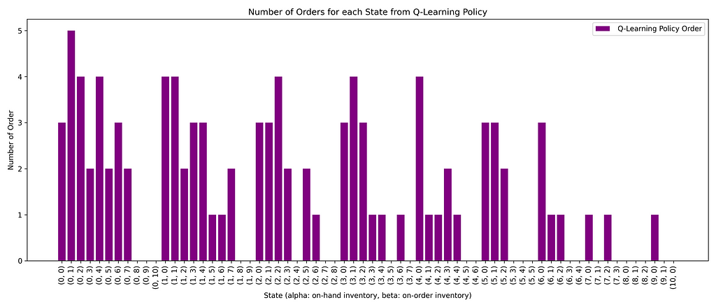 Number of order (y-axis) for each state (x-axis) found from Q-learning policy — Image Source: Author
A couple of learnings can be gained by looking at the plot. First, as we go toward the right, we see that the number of orders decreases. When we go right, the alpha value increases (in-hand inventory), meaning we need to “order” less, as inventory in place can fulfill the demand. Secondly, When alpha is constant, with increasing beta, we lower the order of new sites. It can be understood that this is due to the fact that when “we have more item “on order” we do not need increase the orders.
Comparing the Q-Learning Policy to the BaseLine Policy
Now that we used Q-learning to find the policy (how many items to order in a given state), we can compare it to the baseline policy (a simple policy). The baseline policy is just to “order up to policy,” which simply means you look at the on-hand inventory and the on-order inventory and order up to “meet the target level.” We can write simple code to write this policy in Python format here:
# Create a simple policydef order_up_to_policy(state, user_capacity, target_level):
alpha, beta = state
max_possible_order = user_capacity - (alpha + beta)
desired_order = max(0, target_level - (alpha + beta))
return min(max_possible_order, desired_order)
In the code, the target_level is the desired value we want to order for inventory. If target_level = user_capacity, then we are filling just to fulfill the inventory. First, we can compare the policies of these different methods. For each state, what will be the “number of orders” if we follow the Simple policy and the one from the Q-learning policy? In the figure below, we plotted the comparison of two policies.
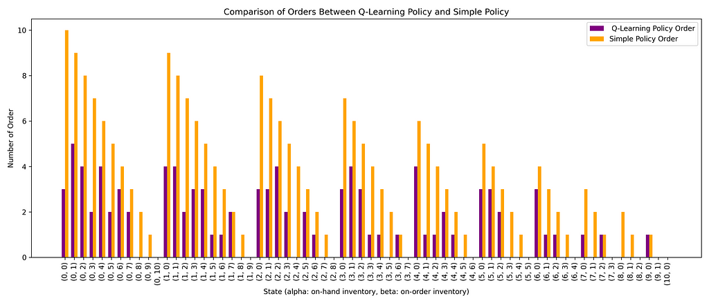 Comparing Ordering policy between Q-Learning and Simple Policy, for each state — Image Source : Author
The simple policy is just to order so that it fulfills the inventory, where the Q-learning policy order is often lower than the simple policy order.
This can be attributed to the fact that “poisson_lambda” here is 4, meaning the demand is much lower than the capacity of the inventory=10, therefore it is not optimal to order “high number of bicycle” as it has a high holding cost.We can also compare the total cumulative rewards you can get when you apply both policies. To do that, we can use the test_policy function of “QLearningInventory” which was especially designed to evaluate policies:
def test_policy(self, policy, episodes):"""
Test a given policy on the environment and calculate the total reward.
Args:
policy (dict): A dictionary mapping states to actions.
episodes (int): The number of episodes to simulate.
Returns:
float: The total reward accumulated over all episodes.
"""
total_reward = 0
alpha_0 = random.randint(0, self.user_capacity)
beta_0 = random.randint(0, self.user_capacity - alpha_0)
state = (alpha_0, beta_0) # Initialize the state
for _ in range(episodes):
action = policy.get(state, 0)
next_state, reward = self.simulate_transition_and_reward(state, action)
total_reward += reward
state = next_state
return total_reward
The way the function works is it starts randomly with a new state (state = (alpha_0, beta_0); then for that state, you get action (number of order) for that state from policy, you act and see the reward, and next state, and the process continues as total number of episodes, while you collect the total reward.
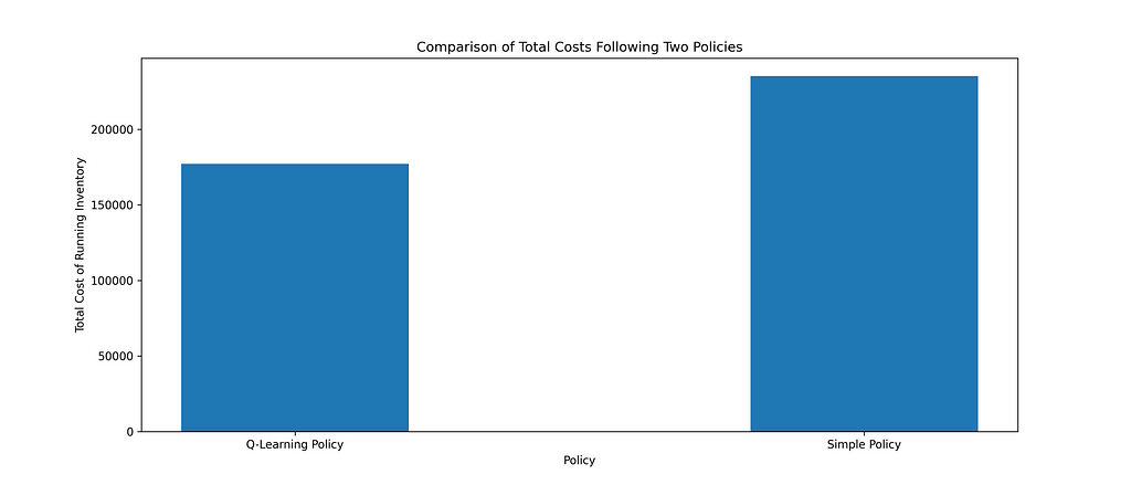 Total costs of manging Inventory, following Q-Learnng policy and Simple policy — Image Source Author
The plot above compares the total cost of managing inventory when we follow the “Q-Learning” and “Simple Policy”. The aim is to mimimize the cost of running inventory. Since the ‘reward’ in our model represents this cost, we added total cost = -total reward.
Running the inventory with the Q-Learning policy will lead to lower costs compared to the Simple policy.Code in GitHub
The full code for this blog can be found in the GitHub repository here.
Summary and Main Takeaways
In this post, we worked on how reinforcement learning (Q-Learning specifically) can be used to optimize inventory management. We were able to develop a Q-learning algorithm that learns the optimal ordering policy through interaction with the environment (uncertainty). Here, the environment was the “random” demand of the customers (buyers of bikes), and the state was the current inventory status (alpha, beta). The Q-learning algorithm was able to learn the optimal policy that minimizes the total cost of inventory management.
Main Takeaways
- Q-Learning: A model-free reinforcement learning algorithm, Q-learning, can be used to find the optimal inventory policy without requiring a complete model of the environment.
- State Representation: The state in inventory management is represented by the current on-hand inventory and on-order inventory state = (α, β).
- Cost Reduction: We can see that the Q-learning policy leads to lower costs compared to the simple policy of ordering up to capacity.
- Flexibility: The Q-learning approach is quite flexible and can be applied to the case of we have past data of demand, or we can interact with the environment to learn the optimal policy.
- Data-Driven Decisions: As we showed, the reinforcement learning (RL) approach does not require any prior knowledge on the model of environment , as it is learning from the data.
References
[1] A. Rao, T. Jelvis, Foundations of Reinforcement Learning with Applications in Finance (2022).
[2] S. Sutton, A. Barto, Reinforcement Learning: An Introduction (2018).
[3] W. B. Powell, Sequential Decision Analytics and Modeling: Modeling with Python (2022).
[4] R. B. Bratvold, Making Good Decisions (2010).
Optimizing Inventory Management with Reinforcement Learning: A Hands-on Python Guide was originally published in Towards Data Science on Medium, where people are continuing the conversation by highlighting and responding to this story.


 English (US)