 2 days ago
3
2 days ago
3
Club.noww.in
To curate, or not to curate, that is the question
 AI image created on MidJourney V6.1 by the author.
Time series forecasting is a powerful tool in data science, offering insights into future trends based on historical patterns. In our previous article, we explored how making your time series stationary automatically can significantly enhance model performance. But stationarity is just one piece of the puzzle. As we continue to refine our forecasting models, another crucial question arises: how do we handle the multitude of features our data may present?
As you work with time series data, you’ll often find yourself with many potential features to include in your model. While it’s tempting to use all available data, adding more features isn’t always better. It can make your model more complex and slower to train, without necessarily improving its performance.
You might be wondering: is it important to simplify the feature set and what are the techniques available out there? That’s exactly what we’ll discuss in this article.
Here’s a quick summary of what will be covered:
- Feature reduction in time series — We’ll explain the concept of feature reduction in time series analysis and why it matters.
- Practical implementation guide — Using Python, we’ll walk through evaluating and selecting features for your time series model, providing hands-on tools to optimize your approach. We’ll also assess whether trimming down features is necessary for our forecasting models.
Once you’re familiar with techniques like stationarity and feature reduction as explained in this article, and you’re looking to elevate your models even further? Check out this article on using a custom validation loss in your deep learning model to get better stock forecasts — it’s a great next step!
Feature reduction in time series : a simple explanation
Feature reduction is like cleaning up your workspace to make it easier to find what you need. In time series analysis, it means cutting down the number of input variables (features) that your model uses to make predictions. The goal is to simplify the model while retaining its predictive power. This is important because too many and correlated features can make your model complicated, slow, and less accurate.
Specifically, simplifying the feature set can :
- Reduced complexity: Fewer features means a simpler model, which is often faster to train and use.
- Improved generalization: By removing noise, eliminating correlated features and focusing on key information, it helps the model to learn the true underlying patterns rather than memorizing redundant information. This enhances the model’s ability to generalize its predictions to different datasets.
- Easier interpretation: A model with fewer features is often easier for humans to understand and explain.
- Computational efficiency: Fewer features requires less memory and processing power, which can be crucial for large datasets or real-time applications.
It’s also important to note that most time series packages in Python for forecasting don’t perform feature reduction automatically. This is a step you typically need to handle on your own before using these packages.
To better understand these concepts, let’s walk through a practical example using real-world daily data from the Federal Reserve Economic Data (FRED) database. We’ll skip the data retrieval process here, as we’ve already covered how to get free and reliable data from the FRED API in a previous article. You can get the data we’ll be using this script. Once you’ve fetched the data :
- Create adata directory in your current directory
- Copy the data in your directory
Now that we have our data, let’s dive into our feature reduction example.
We’ve previously demonstrated how to clean the daily data fetched from the FRED API in another article, so we’ll skip that process here and use the processed_dataframes(list of dataframes) that resulted from the steps outlined in that article.
import pandas as pdimport os
import warnings
warnings.filterwarnings("ignore")
def is_sp500(df):
last_date = df['ds'].max()
last_value = float(df.loc[df['ds'] == last_date, 'value'].iloc[0])
return 5400 <= last_value <= 5650
initial_model_train = None
for i, df in enumerate(processed_dataframes):
if df['value'].isna().any():
continue
if is_sp500(df):
initial_model_train = df
break
TRAIN_SIZE = .90
START_DATE = '2018-10-01'
END_DATE = '2024-09-05'
initial_model_train = initial_model_train.rename(columns={'value': 'price'}).reset_index(drop=True)
initial_model_train['unique_id'] = 'SPY'
initial_model_train['price'] = initial_model_train['price'].astype(float)
initial_model_train['y'] = initial_model_train['price'].pct_change()
initial_model_train = initial_model_train[initial_model_train['ds'] > START_DATE].reset_index(drop=True)
combined_df_all = pd.concat([df.drop(columns=['ds']) for df in processed_dataframes], axis=1)
combined_df_all.columns = [f'value_{i}' for i in range(len(processed_dataframes))]
rows_to_keep = len(initial_model_train)
combined_df_all = combined_df_all.iloc[-rows_to_keep:].reset_index(drop=True)
train_size = int(len(initial_model_train)*TRAIN_SIZE)
initial_model_test = initial_model_train[train_size:]
initial_model_train = initial_model_train[:train_size]
combined_df_test = combined_df_all[train_size:]
combined_df_train = combined_df_all[:train_size]
You might be wondering why we’ve divided our data into training and testing sets? The reason is to ensure that there is no data leakage before applying any transformation or reduction technique.
initial_model_data contains the S&P 500 daily prices (stored originally processed_dataframes), which will be the data we’ll be trying to forecast.
Then, we need to ensure our data is stationary. For a detailed explanation on how to automatically make your data stationary and improve your model by 20%, refer to this article.
import numpy as npfrom statsmodels.tsa.stattools import adfuller
P_VALUE = 0.05
def replace_inf_nan(series):
if np.isnan(series.iloc[0]) or np.isinf(series.iloc[0]):
series.iloc[0] = 0
mask = np.isinf(series) | np.isnan(series)
series = series.copy()
series[mask] = np.nan
series = series.ffill()
return series
def safe_convert_to_numeric(series):
return pd.to_numeric(series, errors='coerce')
tempo_df = pd.DataFrame()
stationary_df_train = pd.DataFrame()
stationary_df_test = pd.DataFrame()
value_columns = [col for col in combined_df_all.columns if col.startswith('value_')]
transformations = ['first_diff', 'pct_change', 'log', 'identity']
def get_first_diff(numeric_series):
return replace_inf_nan(numeric_series.diff())
def get_pct_change(numeric_series):
return replace_inf_nan(numeric_series.pct_change())
def get_log_transform(numeric_series):
return replace_inf_nan(np.log(numeric_series.replace(0, np.nan)))
def get_identity(numeric_series):
return numeric_series
for index, val_col in enumerate(value_columns):
numeric_series = safe_convert_to_numeric(combined_df_train[val_col])
numeric_series_all = safe_convert_to_numeric(combined_df_all[val_col])
if numeric_series.isna().all():
continue
valid_transformations = []
tempo_df['first_diff'] = get_first_diff(numeric_series)
tempo_df['pct_change'] = get_pct_change(numeric_series)
tempo_df['log'] = get_log_transform(numeric_series)
tempo_df['identity'] = get_identity(numeric_series)
for transfo in transformations:
tempo_df[transfo] = replace_inf_nan(tempo_df[transfo])
series = tempo_df[transfo].dropna()
if len(series) > 1 and not (series == series.iloc[0]).all():
result = adfuller(series)
if result[1] < P_VALUE:
valid_transformations.append((transfo, result[0], result[1]))
if valid_transformations:
if any(transfo == 'identity' for transfo, _, _ in valid_transformations):
chosen_transfo = 'identity'
else:
chosen_transfo = min(valid_transformations, key=lambda x: x[1])[0]
if chosen_transfo == 'first_diff':
stationary_df_train[val_col] = get_first_diff(numeric_series_all)
elif chosen_transfo == 'pct_change':
stationary_df_train[val_col] = get_pct_change(numeric_series_all)
elif chosen_transfo == 'log':
stationary_df_train[val_col] = get_log_transform(numeric_series_all)
else:
stationary_df_train[val_col] = get_identity(numeric_series_all)
else:
print(f"No valid transformation found for {val_col}")
stationary_df_test = stationary_df_train[train_size:]
stationary_df_train = stationary_df_train[:train_size]
initial_model_train = initial_model_train.iloc[1:].reset_index(drop=True)
stationary_df_train = stationary_df_train.iloc[1:].reset_index(drop=True)
last_train_index = stationary_df_train.index[-1]
stationary_df_test = stationary_df_test.loc[last_train_index + 1:].reset_index(drop=True)
initial_model_test = initial_model_test.loc[last_train_index + 1:].reset_index(drop=True)
Then, we will count the number of variables that have at least a 95% correlation coefficient with another variable.
CORR_COFF = .95corr_matrix = stationary_df_train.corr().abs()
mask = np.triu(np.ones_like(corr_matrix, dtype=bool), k=1)
high_corr = corr_matrix.where(mask).stack()
high_corr = high_corr[high_corr >= CORR_COFF]
unique_cols = set(high_corr.index.get_level_values(0)) | set(high_corr.index.get_level_values(1))
num_high_corr_cols = len(unique_cols)
print(f"\n{num_high_corr_cols}/{stationary_df_train.shape[1]} variables have ≥{int(CORR_COFF*100)}% "
f"correlation with another variable.\n")
 Number of variables highly correlated. Image by the author.
Having 260 out of 438 variables that have a correlation of 95% or more with at least another variable can be an issue. It indicates significant multicollinearity in the dataset. This redundancy can lead to several issues:
- It complicates the model without adding substantial new information
- Potentially causes instability in coefficient estimates
- Increases the risk of overfitting
- Makes interpretation of individual variable impacts challenging
Feature evaluation and selection
We understand that feature reduction can be important, but how do we perform it? Which techniques should we use? These are the questions we’ll explore now.
The first technique we’ll examine is Principal Component Analysis (PCA). It’s a common and an effective dimensionality reduction technique. PCA identifies linear relationships between features and retains the principal components that explain a predetermined percentage of the variance in the original dataset. In our use case, we’ve set the EXPLAINED_VARIANCE threshold to 90%.
from sklearn.preprocessing import StandardScalerfrom sklearn.decomposition import PCA
EXPLAINED_VARIANCE = .9
MIN_VARIANCE = 1e-10
X_train = stationary_df_train.values
scaler = StandardScaler()
X_train_scaled = scaler.fit_transform(X_train)
pca = PCA(n_components=EXPLAINED_VARIANCE, svd_solver='full')
X_train_pca = pca.fit_transform(X_train_scaled)
components_to_keep = pca.explained_variance_ > MIN_VARIANCE
X_train_pca = X_train_pca[:, components_to_keep]
pca_df_train = pd.DataFrame(
X_train_pca,
columns=[f'PC{i+1}' for i in range(X_train_pca.shape[1])]
)
X_test = stationary_df_test.values
X_test_scaled = scaler.transform(X_test)
X_test_pca = pca.transform(X_test_scaled)
X_test_pca = X_test_pca[:, components_to_keep]
pca_df_test = pd.DataFrame(
X_test_pca,
columns=[f'PC{i+1}' for i in range(X_test_pca.shape[1])]
)
print(f"\nOriginal number of features: {stationary_df_train.shape[1]}")
print(f"Number of components after PCA: {pca_df_train.shape[1]}\n")
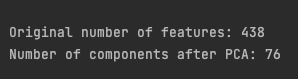 Feature reduction using Principal Component Analysis. Image by the author.
It’s an impressive: only 76 components out of 438 features remaining after the reduction while keeping 90% of the variance explained! Now let’s move to a non-linear reduction technique.
The Temporal Fusion Transformers (TFT) is an advanced model for time series forecasting. It includes the Variable Selection Network (VSN), which is a key component of the model. It’s specifically designed to automatically identify and focus on the most relevant features within a dataset. It achieves this by assigning learned weights to each input variable, effectively highlighting which features contribute most to the predictive task.
This VSN-based approach will be our second reduction technique. We’ll implement it using PyTorch Forecasting, which allows us to leverage the Variable Selection Network from the TFT model.
We’ll use a basic configuration. Our goal isn’t to create the highest-performing model possible, but rather to identify the most relevant features while using minimal resources.
from pytorch_forecasting import TemporalFusionTransformer, TimeSeriesDataSetfrom pytorch_forecasting.metrics import QuantileLoss
from lightning.pytorch.callbacks import EarlyStopping
import lightning.pytorch as pl
import torch
pl.seed_everything(42)
max_encoder_length = 32
max_prediction_length = 1
VAL_SIZE = .2
VARIABLES_IMPORTANCE = .8
model_data_feature_sel = initial_model_train.join(stationary_df_train)
model_data_feature_sel = model_data_feature_sel.join(pca_df_train)
model_data_feature_sel['price'] = model_data_feature_sel['price'].astype(float)
model_data_feature_sel['y'] = model_data_feature_sel['price'].pct_change()
model_data_feature_sel = model_data_feature_sel.iloc[1:].reset_index(drop=True)
model_data_feature_sel['group'] = 'spy'
model_data_feature_sel['time_idx'] = range(len(model_data_feature_sel))
train_size_vsn = int((1-VAL_SIZE)*len(model_data_feature_sel))
train_data_feature = model_data_feature_sel[:train_size_vsn]
val_data_feature = model_data_feature_sel[train_size_vsn:]
unknown_reals_origin = [col for col in model_data_feature_sel.columns if col.startswith('value_')] + ['y']
timeseries_config = {
"time_idx": "time_idx",
"target": "y",
"group_ids": ["group"],
"max_encoder_length": max_encoder_length,
"max_prediction_length": max_prediction_length,
"time_varying_unknown_reals": unknown_reals_origin,
"add_relative_time_idx": True,
"add_target_scales": True,
"add_encoder_length": True
}
training_ts = TimeSeriesDataSet(
train_data_feature,
**timeseries_config
)
The VARIABLES_IMPORTANCE threshold is set to 0.8, which means we'll retain features in the top 80th percentile of importance as determined by the Variable Selection Network (VSN). For more information about the Temporal Fusion Transformers (TFT) and its parameters, please refer to the documentation.
Next, we’ll train the TFT model.
if torch.cuda.is_available():accelerator = 'gpu'
num_workers = 2
else :
accelerator = 'auto'
num_workers = 0
validation = TimeSeriesDataSet.from_dataset(training_ts, val_data_feature, predict=True, stop_randomization=True)
train_dataloader = training_ts.to_dataloader(train=True, batch_size=64, num_workers=num_workers)
val_dataloader = validation.to_dataloader(train=False, batch_size=64*5, num_workers=num_workers)
tft = TemporalFusionTransformer.from_dataset(
training_ts,
learning_rate=0.03,
hidden_size=16,
attention_head_size=2,
dropout=0.1,
loss=QuantileLoss()
)
early_stop_callback = EarlyStopping(monitor="val_loss", min_delta=1e-5, patience=5, verbose=False, mode="min")
trainer = pl.Trainer(max_epochs=20, accelerator=accelerator, gradient_clip_val=.5, callbacks=[early_stop_callback])
trainer.fit(
tft,
train_dataloaders=train_dataloader,
val_dataloaders=val_dataloader
)
We intentionally set max_epochs=20 so the model doesn’t train too long. Additionally, we implemented an early_stop_callback that halts training if the model shows no improvement for 5 consecutive epochs (patience=5).
Finally, using the best model obtained, we select the 80th percentile of the most important features as determined by the VSN.
best_model_path = trainer.checkpoint_callback.best_model_pathbest_tft = TemporalFusionTransformer.load_from_checkpoint(best_model_path)
raw_predictions = best_tft.predict(val_dataloader, mode="raw", return_x=True)
def get_top_encoder_variables(best_tft,interpretation):
encoder_importances = interpretation["encoder_variables"]
sorted_importances, indices = torch.sort(encoder_importances, descending=True)
cumulative_importances = torch.cumsum(sorted_importances, dim=0)
threshold_index = torch.where(cumulative_importances > VARIABLES_IMPORTANCE)[0][0]
top_variables = [best_tft.encoder_variables[i] for i in indices[:threshold_index+1]]
if 'relative_time_idx' in top_variables:
top_variables.remove('relative_time_idx')
return top_variables
interpretation= best_tft.interpret_output(raw_predictions.output, reduction="sum")
top_encoder_vars = get_top_encoder_variables(best_tft,interpretation)
print(f"\nOriginal number of features: {stationary_df_train.shape[1]}")
print(f"Number of features after Variable Selection Network (VSN): {len(top_encoder_vars)}\n")
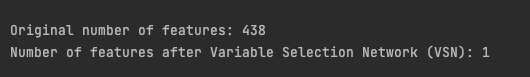 Feature reduction using Variable Selection Network. Image by the author.
The original dataset contained 438 features, which were then reduced to 1 feature only after applying the VSN method! This drastic reduction suggests several possibilities:
- Many of the original features may have been redundant.
- The feature selection process may have oversimplified the data.
- Using only the target variable’s historical values (autoregressive approach) might perform as well as, or possibly better than, models incorporating exogenous variables.
Evaluating feature reduction techniques
In this final section, we compare out reduction techniques applied to our model. Each method is tested while maintaining identical model configurations, varying only the features subjected to reduction.
We’ll use TiDE, a small state-of-the-art Transformer-based model. We’ll use the implementation provided by NeuralForecast. Any model from NeuralForecast here would work as long as it allows exogenous historical variables.
We’ll train and test two models using daily SPY (S&P 500 ETF) data. Both models will have the same:
- Train-test split ratio
- Hyperparameters
- Single time series (SPY)
- Forecasting horizon of 1 step ahead
The only difference between the models will be the feature reduction technique. That’s it!
- First model: Original features (no feature reduction)
- Second model: Feature reduction using PCA
- Third model: Feature reduction using VSN
This setup allows us to isolate the impact of each feature reduction technique on model performance.
First we train the 3 models with the same configuration except for the features.
from neuralforecast.models import TiDEfrom neuralforecast import NeuralForecast
train_data = initial_model_train.join(stationary_df_train)
train_data = train_data.join(pca_df_train)
test_data = initial_model_test.join(stationary_df_test)
test_data = test_data.join(pca_df_test)
hist_exog_list_origin = [col for col in train_data.columns if col.startswith('value_')] + ['y']
hist_exog_list_pca = [col for col in train_data.columns if col.startswith('PC')] + ['y']
hist_exog_list_vsn = top_encoder_vars
tide_params = {
"h": 1,
"input_size": 32,
"scaler_type": "robust",
"max_steps": 500,
"val_check_steps": 20,
"early_stop_patience_steps": 5
}
model_original = TiDE(
**tide_params,
hist_exog_list=hist_exog_list_origin,
)
model_pca = TiDE(
**tide_params,
hist_exog_list=hist_exog_list_pca,
)
model_vsn = TiDE(
**tide_params,
hist_exog_list=hist_exog_list_vsn,
)
nf = NeuralForecast(
models=[model_original, model_pca, model_vsn],
freq='D'
)
val_size = int(train_size*VAL_SIZE)
nf.fit(df=train_data,val_size=val_size,use_init_models=True)
Then, we make the predictions.
from tabulate import tabulatey_hat_test_ret = pd.DataFrame()
current_train_data = train_data.copy()
y_hat_ret = nf.predict(current_train_data)
y_hat_test_ret = pd.concat([y_hat_test_ret, y_hat_ret.iloc[[-1]]])
for i in range(len(test_data) - 1):
combined_data = pd.concat([current_train_data, test_data.iloc[[i]]])
y_hat_ret = nf.predict(combined_data)
y_hat_test_ret = pd.concat([y_hat_test_ret, y_hat_ret.iloc[[-1]]])
current_train_data = combined_data
predicted_returns_original = y_hat_test_ret['TiDE'].values
predicted_returns_pca = y_hat_test_ret['TiDE1'].values
predicted_returns_vsn = y_hat_test_ret['TiDE2'].values
predicted_prices_original = []
predicted_prices_pca = []
predicted_prices_vsn = []
for i in range(len(predicted_returns_pca)):
if i == 0:
last_true_price = train_data['price'].iloc[-1]
else:
last_true_price = test_data['price'].iloc[i-1]
predicted_prices_original.append(last_true_price * (1 + predicted_returns_original[i]))
predicted_prices_pca.append(last_true_price * (1 + predicted_returns_pca[i]))
predicted_prices_vsn.append(last_true_price * (1 + predicted_returns_vsn[i]))
true_values = test_data['price']
methods = ['Original','PCA', 'VSN']
predicted_prices = [predicted_prices_original,predicted_prices_pca, predicted_prices_vsn]
results = []
for method, prices in zip(methods, predicted_prices):
mse = np.mean((np.array(prices) - true_values)**2)
rmse = np.sqrt(mse)
mae = np.mean(np.abs(np.array(prices) - true_values))
results.append([method, mse, rmse, mae])
headers = ["Method", "MSE", "RMSE", "MAE"]
table = tabulate(results, headers=headers, floatfmt=".4f", tablefmt="grid")
print("\nPrediction Errors Comparison:")
print(table)
with open("prediction_errors_comparison.txt", "w") as f:
f.write("Prediction Errors Comparison:\n")
f.write(table)
We forecast the daily returns using the model, then convert these back to prices. This approach allows us to calculate prediction errors using prices and compare the actual prices to the forecasted prices in a plot.
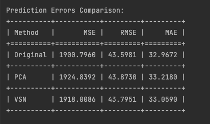 Comparison of prediction errors with different feature reduction techniques. Image by the author.
The similar performance of the TiDE model across both original and reduced feature sets reveals a crucial insight: feature reduction did not lead to improved predictions as one might expect. This suggests potential key issues:
- Information loss: despite aiming to preserve essential data, dimensionality reduction techniques discarded information relevant to the prediction task, explaining the lack of improvement with fewer features.
- Generalization struggles: consistent performance across feature sets indicates the model’s difficulty in capturing underlying patterns, regardless of feature count.
- Complexity overkill: similar results with fewer features suggest TiDE’s sophisticated architecture may be unnecessarily complex. A simpler model, like ARIMA, could potentially perform just as well.
Then, let’s examine the chart to see if we can observe any significant differences among the three forecasting methods and the actual prices.
import matplotlib.pyplot as pltplt.figure(figsize=(12, 6))
plt.plot(train_data['ds'], train_data['price'], label='Training Data', color='blue')
plt.plot(test_data['ds'], true_values, label='True Prices', color='green')
plt.plot(test_data['ds'], predicted_prices_original, label='Predicted Prices', color='red')
plt.legend()
plt.title('SPY Price Forecast Using All Original Feature')
plt.xlabel('Date')
plt.ylabel('SPY Price')
plt.savefig('spy_forecast_chart_original.png', dpi=300, bbox_inches='tight')
plt.close()
plt.figure(figsize=(12, 6))
plt.plot(train_data['ds'], train_data['price'], label='Training Data', color='blue')
plt.plot(test_data['ds'], true_values, label='True Prices', color='green')
plt.plot(test_data['ds'], predicted_prices_pca, label='Predicted Prices', color='red')
plt.legend()
plt.title('SPY Price Forecast Using PCA Dimensionality Reduction')
plt.xlabel('Date')
plt.ylabel('SPY Price')
plt.savefig('spy_forecast_chart_pca.png', dpi=300, bbox_inches='tight')
plt.close()
plt.figure(figsize=(12, 6))
plt.plot(train_data['ds'], train_data['price'], label='Training Data', color='blue')
plt.plot(test_data['ds'], true_values, label='True Prices', color='green')
plt.plot(test_data['ds'], predicted_prices_vsn, label='Predicted Prices', color='red')
plt.legend()
plt.title('SPY Price Forecast Using VSN')
plt.xlabel('Date')
plt.ylabel('SPY Price')
plt.savefig('spy_forecast_chart_vsn.png', dpi=300, bbox_inches='tight')
plt.close()
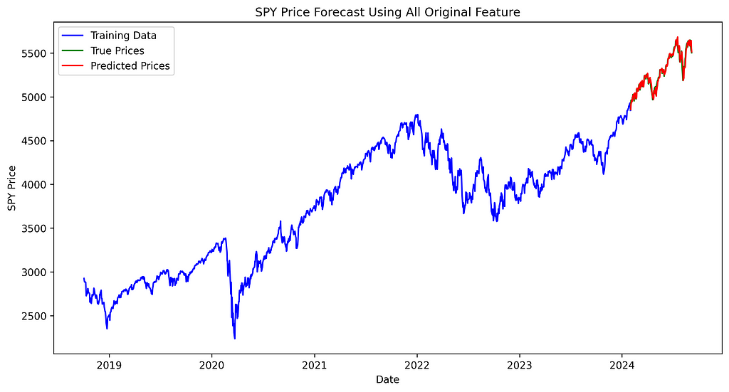 SPY price forecast using all original features. Image created by the author.
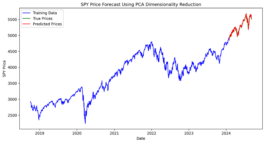 SPY price forecast using PCA. Image created by the author.
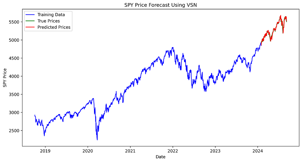 SPY price forecast using VSN. Image created by the author.
The difference between true and predicted prices appears consistent across all three models, with no noticeable variation in performance between them.
Conclusion
We did it! We explored the importance of feature reduction in time series analysis and provided a practical implementation guide:
- Feature reduction aims to simplify models while maintaining predictive power. Benefits include reduced complexity, improved generalization, easier interpretation, and computational efficiency.
- We demonstrated two reduction techniques using FRED data:
- Principal Component Analysis (PCA), a linear dimensionality reduction method, reduced features from 438 to 76 while retaining 90% of explained variance.
- Variable Selection Network (VSN) from the Temporal Fusion Transformers, a non-linear approach, drastically reduced features to just 1 using an 80th percentile importance threshold.
- Evaluation using TiDE models showed similar performance across original and reduced feature sets, suggesting feature reduction may not always improve forecasting performance. This could be due to information loss during reduction, the model’s difficulty in capturing underlying patterns, or the possibility that a simpler model might be equally effective for this particular forecasting task.
On a final note, we didn’t explore all feature reduction techniques, such as SHAP (SHapley Additive exPlanations), which provides a unified measure of feature importance across various model types. Even if we didn’t improve our model, it’s still better to perform feature curation and compare performance across different reduction methods. This approach helps ensure you’re not discarding valuable information while optimizing your model’s efficiency and interpretability.
In future articles, we’ll apply these feature reduction techniques to more complex models, comparing their impact on performance and interpretability. Stay tuned!
Ready to put these concepts into action? You can find the complete code implementation here.
Liked this article? Show your support!
👏 Clap it up to 50 times
🤝 Send me a LinkedIn connection request to stay in touch
Your support means everything! 🙏
Is Less More? Do Deep Learning Forecasting Models Need Feature Reduction? was originally published in Towards Data Science on Medium, where people are continuing the conversation by highlighting and responding to this story.


 English (US)