Stein’s Paradox

Why the Sample Mean Isn’t Always the Best

Image by Author

Averaging is one of the most fundamental tools in statistics, second only to counting. While its simplicity might make it seem intuitive, averaging plays a central role in many mathematical concepts because of its robust properties. Major results in probability, such as the Law of Large Numbers and the Central Limit Theorem, emphasize that averaging isn’t just convenient — it’s often optimal for estimating parameters. Core statistical methods, like Maximum Likelihood Estimators and Minimum Variance Unbiased Estimators (MVUE), reinforce this notion.

However, this long-held belief was upended in 1956[1] when Charles Stein made a breakthrough that challenged over 150 years of estimation theory.

History

Averaging has traditionally been seen as an effective method for estimating the central tendency of a random variable’s distribution, particularly in the case of a normal distribution. The normal (or Gaussian) distribution is characterized by its bell-shaped curve and two key parameters: the mean (θ) and the standard deviation (σ). The mean indicates the center of the curve, while the standard deviation reflects the spread of the data.

Statisticians often work backward, inferring these parameters from observed data. Gauss demonstrated that the sample mean maximizes the likelihood of observing the data, making it an unbiased estimator — meaning it doesn’t systematically overestimate or underestimate the true mean (θ).

Further developments in statistical theory confirmed the utility of the sample mean, which minimizes the expected squared error when compared to other linear unbiased estimators. Researchers like R.A. Fisher and Jerzy Neyman expanded on these ideas by introducing risk functions, which measure the average squared error for different values of θ. They found that while both the mean and the median have constant risk, the mean consistently delivers lower risk, confirming its superiority.

However, Stein’s theorem showed that when estimating three or more parameters simultaneously, the sample mean becomes inadmissible. In these cases, biased estimators can outperform the sample mean by offering lower overall risk. Stein’s work revolutionized statistical inference, improving accuracy in multi-parameter estimation.

The James-Stein Estimator

The James-Stein[2] estimator is a key tool in the paradox discovered by Charles Stein. It challenges the notion that the sample mean is always the best estimator, particularly when estimating multiple parameters simultaneously. The idea behind the James-Stein estimator is to “shrink” individual sample means toward a central value (the grand mean), which reduces the overall estimation error.

To clarify this, let’s start by considering a vector x representing the sample means of several variables (not necessarily independent). If we take the average of all these means, we get a single value, denoted by μ, which we refer to as the grand mean. The James-Stein estimator works by moving each sample mean closer to this grand mean, reducing their variance.

The general formula[3] for the James-Stein estimator is:

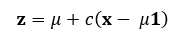
Where:

• x is the sample mean vector.
• μ is the grand mean (the average of the sample means).
• c is a shrinkage factor that lies between 0 and 1. It determines how much we pull the individual means toward the grand mean.

The goal here is to reduce the distance between the individual sample means and the grand mean. For example, if one sample mean is far from the grand mean, the estimator will shrink it toward the center, smoothing out the variation in the data.

The value of c, the shrinkage factor, depends on the data and what is being estimated. A sample mean vector follows a multivariate normal distribution, so if this is what we are trying to estimate, the formula becomes:

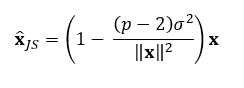
Where:

• p is the number of parameters being estimated (the length of x).
• σ² is the variance of the sample mean vector x.
• The term (p — 2)/||x||² adjusts the amount of shrinkage based on the data’s variance and the number of parameters.

Key Assumptions and Adjustments

One key assumption for using the James-Stein estimator is that the variance σ² is the same for all variables, which is often not realistic in real-world data. However, this assumption can be mitigated by standardizing the data, so all variables have the same variance. Alternatively, you can average the individual variances into one pooled estimate. This approach works especially well with larger datasets, where the variance differences tend to diminish as sample size increases.

Once the data is standardized or pooled, the shrinkage factor can be applied to adjust each sample mean appropriately.

Choosing the Shrinkage Factor

The shrinkage factor c is crucial because it controls how much the sample means are pulled toward the grand mean. A value of c close to 1 means little to no shrinkage, which resembles the behavior of the regular sample mean. Conversely, a c close to 0 means significant shrinkage, pulling the sample means almost entirely toward the grand mean.

The optimal value of c depends on the specific data and the parameters being estimated, but the general guideline is that the more parameters there are (i.e., larger p), the more shrinkage is beneficial, as this reduces the risk of over fitting to noisy data.

Implementing the James-Stein Estimator in Code

Here are the James-Stein estimator functions in R, Python, and Julia:

## R ##
james_stein_estimator <- function(Xbar, sigma2 = 1) {
p <- length(Xbar)
norm_X2 <- sum(Xbar^2)
shrinkage_factor <- max(0, 1 - (p - 2) * mean(sigma2) / norm_X2)
return(shrinkage_factor * Xbar)
}

## Python ##
import numpy as np

def james_stein_estimator(Xbar, sigma2=1):
p = len(Xbar)
norm_X2 = np.sum(Xbar**2)
shrinkage_factor = max(0, 1 - (p - 2) * np.mean(sigma2) / norm_X2)
return shrinkage_factor * Xbar

## Julia ##
function james_stein_estimator(Xbar, sigma2=1)
p = length(Xbar)
norm_X2 = sum(Xbar.^2)
shrinkage_factor = max(0, 1 - (p - 2) * mean(sigma2) / norm_X2)
return shrinkage_factor * Xbar
end

Example

To demonstrate the versatility of this technique, I will generate a 6-dimensional data set with each column containing numerical data from various random distributions. Here are the specific distributions and parameters of each I will be using:

X1 ~ t-distribution (ν = 3)
X2 ~ Binomial (n = 10, p = 0.4)
X3 ~ Gamma (α = 3, β = 2)
X4 ~ Uniform (a = 0, b = 1)
X5 ~ Exponential (λ = 50)
X6 ~ Poisson (λ = 2)

Note each column in this data set contains independent variables, in that no column should be correlated with another since they were created independently. This is not a requirement to use this method. It was done this way simply for simplicity and to demonstrate the paradoxical nature of this result. If you’re not entirely familiar with any or all of these distributions, I’ll include a simple visual of each of the univariate columns of the randomly generated data. This is simply one iteration of 1,000 generated random variables from each of the aforementioned distributions.

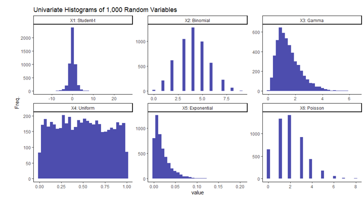
It should be clear from the histograms above that not all of these variables follow a normal distribution implying the dataset as a whole is not multivariate normal.

Since the true distributions of each are known, we know the true averages of each. The average of this multivariate dataset can be expressed in vector form with each row entry representing the average of the variable respectively. In this example,

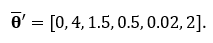
Knowing the true averages of each variable will allow us to be able to measure how close the sample mean, or James Stein estimator gets implying the closer the better. Below is the experiment I ran in R code which generated each of the 6 random variables and tested against the true averages using the Mean Squared Error. This experiment was then ran 10,000 times using four different sample sizes: 5, 50, 500, and 5,000.

set.seed(42)
## Function to calculate Mean Squared Error ##
mse <- function(x, true_value)
return( mean( (x - true_value)^2 ) )
## True Average ##
mu <- c(0, 4, 1.5, 0.5, 0.02, 2)
## Store Average and J.S. Estimator Errors ##
Xbar.MSE <- list(); JS.MSE <- list()
for(n in c(5, 50, 500, 5000)){ # Testing sample sizes of 5, 30, 200, and 5,000
for(i in 1:1e4){ # Performing 10,000 iterations

## Six Random Variables ##
X1 <- rt(n, df = 3)
X2 <- rbinom(n, size = 10, prob = 0.4)
X3 <- rgamma(n, shape = 3, rate = 2)
X4 <- runif(n)
X5 <- rexp(n, rate = 50)
X6 <- rpois(n, lambda = 2)

X <- cbind(X1, X2, X3, X4, X5, X6)

## Estimating Std. Dev. of Each and Standardizing Data ##
sigma <- apply(X, MARGIN = 2, FUN = sd)

## Sample Mean ##
Xbar <- colMeans(X)

## J.S. Estimator ##
JS.Xbar <- james_stein_estimator(Xbar=Xbar, sigma2=sigma/n)

Xbar.MSE[[as.character(n)]][i] <- mse(Xbar, mu)
JS.MSE[[as.character(n)]][i] <- mse(JS.Xbar, mu)

}
}
sapply(Xbar.MSE, mean) # Avg. Sample Mean MSE
sapply(JS.MSE, mean) # Avg. James-Stein MSE

From all 40,000 trails, the total average MSE of each sample size is computed by running the last two lines. The results of each can be seen in the table below.

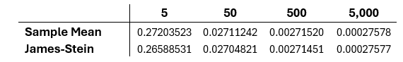
The results of this of this simulation show that the James-Stein estimator is consistently better than the sample mean using the MSE, but that this difference decreases as the sample size increases.

Conclusion

The James-Stein estimator demonstrates a paradox in estimation: it is possible to improve estimates by incorporating information from seemingly independent variables. While the difference in MSE might be negligible for large sample sizes, this result sparked much debate when it was first introduced. The discovery marked a key turning point in statistical theory, and it remains relevant today for multi-parameter estimation.

If you’d like to explore more, check out this detailed article on Stein’s paradox and other references used to write this document.

References

[1] Stein, C. (1956). Inadmissibility of the usual estimator for the mean of a multivariate normal distribution. Proceedings of the Third Berkeley Symposium on Mathematical Statistics and Probability, 1, 197–206.

[2] Stein, C. (1961). Estimation with quadratic loss. In S. S. Gupta & J. O. Berger (Eds.), Statistical Decision Theory and Related Topics (Vol. 1, pp. 361–379). Academic Press.

[3] Efron, B., & Morris, C. (1977). Stein’s paradox in statistics. Scientific American, 236(5), 119–127

---

Stein’s Paradox was originally published in Towards Data Science on Medium, where people are continuing the conversation by highlighting and responding to this story.