 20 hours ago
3
20 hours ago
3
Club.noww.in
It’s now easier than ever to train your own computer vision models on custom datasets using Python, the command line, or Google Colab.
 Image created by author using ChatGPT Auto.
Ultralytics’ cutting-edge YOLOv8 model is one of the best ways to tackle computer vision while minimizing hassle. It is the 8th and latest iteration of the YOLO (You Only Look Once) series of models from Ultralytics, and like the other iterations uses a convolutional neural network (CNN) to predict object classes and their bounding boxes. The YOLO series of object detectors has become well known for being accurate and quick, and provides a platform built on top of PyTorch that simplifies much of the process of creating models from scratch.
Importantly, YOLOv8 is also a very flexible model. That is, it can be trained on a variety of platforms, using any dataset of your choice, and the prediction model can be ran from many sources. This guide will act as a comprehensive tutorial covering the many different ways to train and run YOLOv8 models, as well as the strengths and limitations of each method that will be most relevant in helping you choose the most appropriate procedure depending on your hardware and dataset.
Note: all images that were used in the creation of this example dataset were taken by the author.
Environment
To get started with training our YOLOv8 model, the first step is to decide what kind of environment we want to train our model in (keep in mind that training and running the model are separate tasks).
The environments that are available for us to choose can largely be broken down into two categories: local-based and cloud-based.
With local-based training, we are essentially running the process of training directly on our system, using the physical hardware of the device. Within local-based training, YOLOv8 provides us with two options: the Python API and the CLI. There is no real difference in the results or speed of these two options, because the same process is being run under the hood; the only difference is in how the training is setup and run.
On the other hand, cloud-based training allows you to take advantage of the hardware of cloud servers. By using the Internet, you can connect to cloud runtimes and execute code just as you would on your local machine, except now it runs on the cloud hardware.
By far, the most popular cloud platform for machine learning has been Google Colab. It uses a Jupyter notebook format, which allows users to create “cells” in which code snippets can be written and run, and offers robust integrations with Google Drive and Github.
Which environment you decide to use will largely depend on the hardware that is available to you. If you have a powerful system with a high-end NVIDIA GPU, local-based training will likely work well for you. If your local machine’s hardware isn’t up to spec for machine learning, or if you just want more computation power than you have locally, Google Colab may be the way to go.
One of the greatest benefits of Google Colab is that it offers some computing resources for free, but also has a simple upgrade path that allows you to leverage faster computing hardware. Even if you already have a powerful system, you could consider using Google Colab if the faster GPUs offered in their higher tier plans represent a significant performance improvement over your existing hardware. With the free plan, you are limited to the NVIDIA T4, which performs roughly equivalent to an RTX 2070. With higher tier plans, the L4 (about the performance of a 4090) and A100 (about the performance of 2 4090s) are available. Keep in mind when comparing GPUs that the amount of VRAM is the primary determinant of machine learning performance.
Dataset
In order to start training a model, you need lots of data to train it on. Object detection datasets normally consist of a collection of images of various objects, in addition to a “bounding box” around the object that indicates its location within the image.
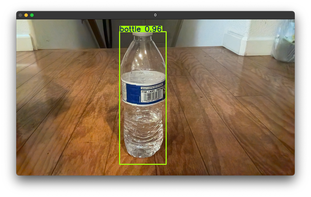 Example of a bounding box around a detected object. Image by author.
YOLOv8-compatible datasets have a specific structure. They are primarily divided into valid, train, and test folders, which are used for validation, training, and testing of the model respectively (the difference between validation and testing is that during validation, the results are used to tune the model to increase its accuracy, whereas during testing, the results are only used to provide a measure of the model’s real-world accuracy).
Within each of these folders the dataset is further divided into two folders: the images and labels folders. The content of these two folders are closely linked with each other.
The images folder, as its name suggests, contains all of the object images of the dataset. These images usually have a square aspect ratio, a low resolution, and a small file size.
The labels folder contains the data of the bounding box’s position and size within each image as well as the type (or class) of object represented by each image. For example:
5 0.8762019230769231 0.09615384615384616 0.24519230769230768 0.1899038461538461511 0.8846153846153846 0.2800480769230769 0.057692307692307696 0.019230769230769232
11 0.796875 0.2668269230769231 0.04807692307692308 0.02403846153846154
17 0.5649038461538461 0.29927884615384615 0.07211538461538461 0.026442307692307692
8 0.48197115384615385 0.39663461538461536 0.06490384615384616 0.019230769230769232
11 0.47716346153846156 0.7884615384615384 0.07932692307692307 0.10576923076923077
11 0.3425480769230769 0.5745192307692307 0.11057692307692307 0.038461538461538464
6 0.43509615384615385 0.5216346153846154 0.019230769230769232 0.004807692307692308
17 0.4855769230769231 0.5264423076923077 0.019230769230769232 0.004807692307692308
2 0.26322115384615385 0.3713942307692308 0.02403846153846154 0.007211538461538462
Each line represents an individual object that is present in the image. Within each line, the first number represents the object’s class, the second and third numbers represent the x- and y-coordinates of the center of the bounding box, and the fourth and fifth numbers represent the width and height of the bounding box.
The data within the images and labels folders are linked together by file names. Every image in the images folder will have a corresponding file in the labels folder with the same file name, and vice versa. Within the dataset, there will always be matching pairs of files within the images and labels folders with the same file name, but with different file extensions; .jpg is used for the images whereas .txt is used for the labels. The data for the bounding box(es) for each object in a .jpg picture is contained in the corresponding .txt file.
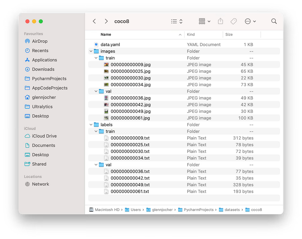 Typical file structure of a YOLOv8-compatible dataset. Source: Ultralytics YOLO Docs (https://docs.ultralytics.com/datasets/detect/#ultralytics-yolo-format)
There are several ways to obtain a YOLOv8-compatible dataset to begin training a model. You can create your own dataset or use a pre-configured one from the Internet. For the purposes of this tutorial, we will use CVAT to create our own dataset and Kaggle to find a pre-configured one.
CVAT
CVAT (cvat.ai) is a annotation tool that lets you create your own datasets by manually adding labels to images and videos.
After creating an account and logging in, the process to start annotating is simple. Just create a project, give it a suitable name, and add the labels for as many types/classes of objects as you want.
 Creating a new project and label on cvat.ai. Video by author.
Create a new task and upload all the images you want to be part of your dataset. Click “Submit & Open”, and a new task should be created under the project, with one job.
 Creating a new task and job on cvat.ai. Video by author.
Opening this job will allow you to start the annotation process. Use the rectangle tool to create bounding boxes and labels for each of the images in your dataset.
 Using the rectangle tool on cvat.ai to create bounding boxes. Video by author.
After annotating all your images, go back to the task and select Actions → Export task dataset, and choose YOLOv8 Detection 1.0 as the Export format. After downloading the task dataset, you will find that it only contains the labels folder and not the images folder (unless you selected the “Save images” option while exporting). You will have to manually create the images folder and move your images there (you may want to first compress your images to a lower resolution e.g. 640x640). Remember to not change the file names as they must match the file names of the .txt files in the labels folder. You will also need to decide how to allocate the images between valid, train, and test (train is the most important out of these).
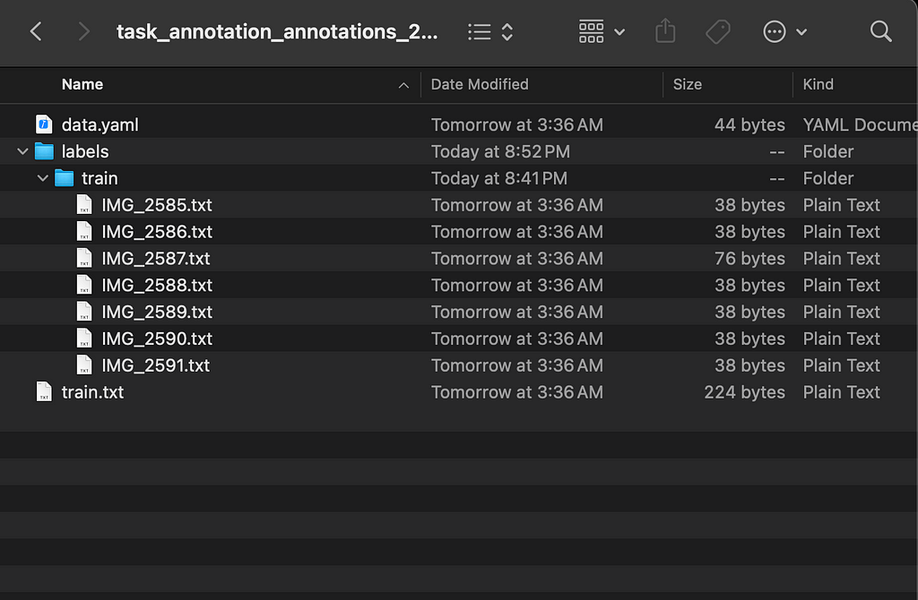 Example dataset exported from cvat.ai. Image by author.
Your dataset is completed and ready to use!
Kaggle
Kaggle (kaggle.com) is one of the largest online data science communities and one of the best websites to explore datasets. You can try finding a dataset you need by simply searching their website, and unless you are looking for something very specific, chances are you will find it. However, many datasets on Kaggle are not in a YOLOv8-compatible format and/or are unrelated to computer vision, so you may want to include “YOLOv8” in your query to refine your search.
You can tell if a dataset is YOLOv8-compatible by the file structure in the dataset’s Data Explorer (on the right side of the page).
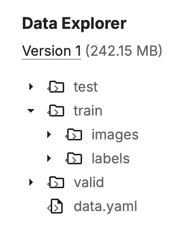 Example of a YOLOv8-compatible dataset on Kaggle. Image by author.
If the dataset is relatively small (a few MB) and/or you are training locally, you can download the dataset directly from Kaggle. However, if you are planning on training with a large dataset on Google Colab, it is better to retrieve the dataset from the notebook itself (more info below).
Training
The training process will differ depending on if you are training locally or on the cloud.
Local
Create a project folder for all the training files. For this tutorial we will call it yolov8-project. Move/copy the dataset to this folder.
Set up a Python virtual environment with required YOLOv8 dependencies:
python3 -m venv venvsource venv/bin/activate
pip3 install ultralytics
Create a file named config.yaml. This is where important dataset information for training will be specified:
path: /Users/oliverma/yolov8-project/dataset/ # absolute path to datasettest: test/images # relative path to test images
train: train/images # relative path to training images
val: val/images # relative path to validation images
# classes
names:
0: bottle
In path put the absolute file path to the dataset’s root directory. You can also use a relative file path, but that will depend on the relative location of config.yaml.
In test, train, and val, put the locations of the images for testing, training, and validation (if you only have train images, just use train/images for all 3).
Under names, specify the name of each class. This information can usually be found in the data.yaml file of any YOLOv8 dataset.
As previously mentioned, both the Python API or the CLI can be used for local training.
Python API
Create another file named main.py. This is where the actual training will begin:
from ultralytics import YOLOmodel = YOLO("yolov8n.yaml")
model.train(data="config.yaml", epochs=100)
By initializing our model as YOLO("yolov8n.yaml") we are essentially creating a new model from scratch. We are using yolov8n because it is the fastest model, but you may also use other models depending on your use case.
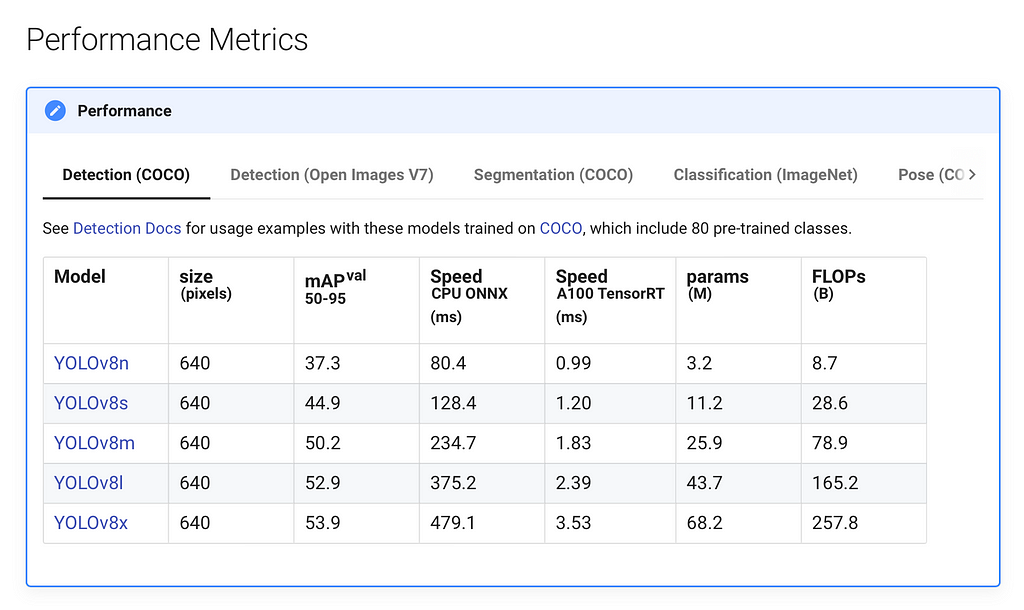 Performance metrics for YOLOv8 variants. Source: Ultralytics YOLO Docs (https://docs.ultralytics.com/models/yolov8/#performance-metrics)
Finally, we train the model and pass in the config file and the number of epochs, or rounds of training. A good baseline is 300 epochs, but you may want to tweak this number depending on the size of your dataset and the speed of your hardware.
There are a few more helpful settings that you may want to include:
- imgsz: resizes all images to the specified amount. For example, imgsz=640 would resize all images to 640x640. This is useful if you created your own dataset and did not resize the images.
- device: specifies which device to train on. By default, YOLOv8 tries to train on GPU and uses CPU training as a fallback, but if you are training on an M-series Mac, you will have to use device="mps" to train with Apple’s Metal Performance Shaders (MPS) backend for GPU acceleration.
For more information on all the training arguments, visit https://docs.ultralytics.com/modes/train/#train-settings.
Your project directory should now look similar to this:
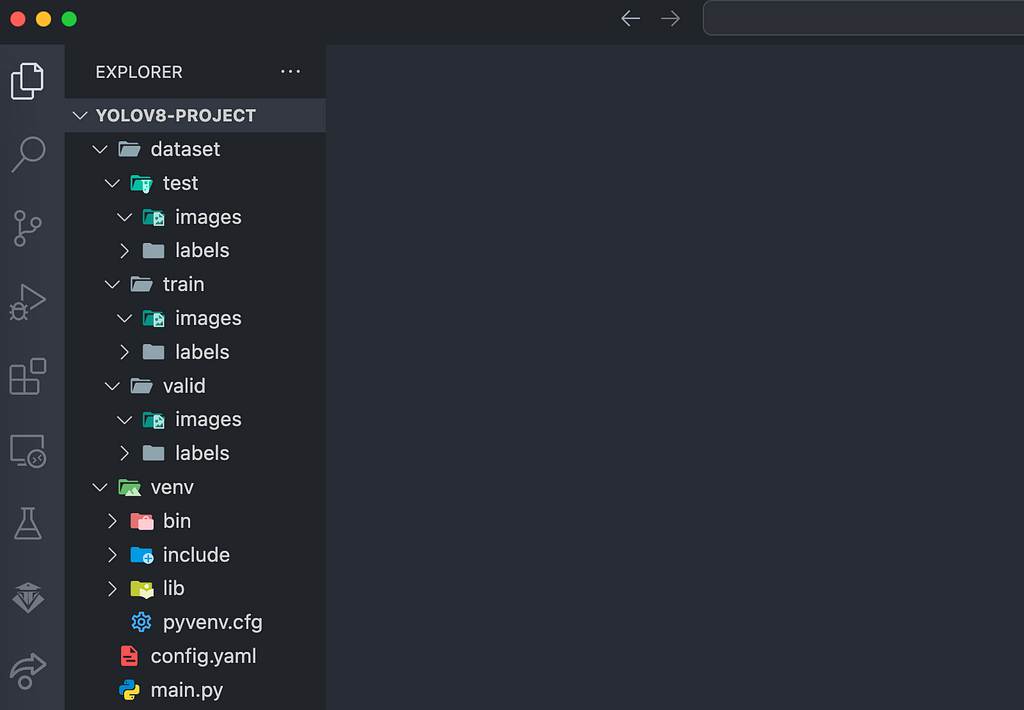 Example file structure of the project directory. Image by author.
We are finally ready to start training our model. Open a terminal in the project directory and run:
python3 main.pyThe terminal will display information about the training progress for each epoch as the training progresses.
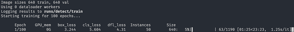 Training progress for each epoch displayed in the terminal. Image by author.
The training results will be saved in runs/detect/train (or train2, train3, etc.). This includes the weights (with a .pt file extension), which will be important for running the model later, as well as results.png which shows many graphs containing relevant training statistics.
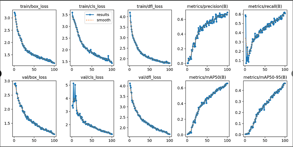 Example graphs from results.png. Image by Author.
CLI
Open a new terminal in the project directory and run this command:
yolo detect train data=config.yaml model=yolov8n.yaml epochs=100This command can be modified with the same arguments as listed above for the Python API. For example:
yolo detect train data=config.yaml model=yolov8n.yaml epochs=300 imgsz=640 device=mpsTraining will begin, and progress will be displayed in the terminal. The rest of the training process is the same as with the Python CLI.
Google Colab
Go to https://colab.research.google.com/ and create a new notebook for training.
Before training, make sure you are connected to a GPU runtime by selecting Change runtime type in the upper-right corner. Training will be extremely slow on a CPU runtime.
 Changing the notebook runtime from CPU to T4 GPU. Video by author.
Before we can begin any training on Google Colab, we first need to import our dataset into the notebook. Intuitively, the simplest way would be to upload the dataset to Google Drive and import it from there into our notebook. However, it takes an exceedingly long amount of time to upload any dataset that is larger than a few MB. The workaround to this is to upload the dataset onto a remote file hosting service (like Amazon S3 or even Kaggle), and pull the dataset directly from there into our Colab notebook.
Import from Kaggle
Here are instructions on how to import a Kaggle dataset directly into a Colab notebook:
In Kaggle account settings, scroll down to API and select Create New Token. This will download a file named kaggle.json.
Run the following in a notebook cell:
!pip install kagglefrom google.colab import files
files.upload()
Upload the kaggle.json file that was just downloaded, then run the following:
!mkdir ~/.kaggle!cp kaggle.json ~/.kaggle/
!chmod 600 ~/.kaggle/kaggle.json
!kaggle datasets download -d [DATASET] # replace [DATASET] with the desired dataset ref
The dataset will download as a zip archive. Use the unzip command to extract the contents:
!unzip dataset.zip -d datasetStart Training
Create a new config.yaml file in the notebook’s file explorer and configure it as previously described. The default working directory in a Colab notebook is /content/, so the absolute path to the dataset will be /content/[dataset folder]. For example:
path: /content/dataset/ # absolute path to datasettest: test/images # relative path to test images
train: train/images # relative path to training images
val: val/images # relative path to validation images
# classes
names:
0: bottle
Make sure to check the file structure of your dataset to make sure the paths specified in config.yaml are accurate. Sometimes datasets will be nestled within multiple levels of folders.
Run the following as cells:
!pip install ultralyticsimport osfrom ultralytics import YOLOmodel = YOLO("yolov8n.yaml")
results = model.train(data="config.yaml", epochs=100)
The previously mentioned arguments used to modify local training settings also apply here.
Similar to local training, results, weights, and graphs will be saved in runs/detect/train.
Running
Regardless of whether you trained locally or on the cloud, predictions must be run locally.
After a model has completed training, there will be two weights located in runs/detect/train/weights, named best.pt and last.pt, which are the weights for the best epoch and the latest epoch, respectively. For this tutorial, we will use best.pt to run the model.
If you trained locally, move best.pt to a convenient location (e.g. our project folder yolov8-project) for running predictions. If you trained on the cloud, download best.pt to your device. On Google Colab, right-click on the file in the notebook’s file explorer and select Download.
 Downloading weights on Google Colab. Video by author.
Similar to local training, predictions can be run either through the Python API or the CLI.
Python API
In the same location as best.pt, create a new file named predict.py:
from ultralytics import YOLOmodel = YOLO("best.pt")
results = model(source=0, show=True, conf=0.25, save=True)
Similar to training, there are many useful arguments that will modify the prediction settings:
- source: controls the input source for the predictions. source=0 sets the webcam as the input source. More info below.
- show: if True , displays the predictions, bounding boxes, and confidences on-screen.
- conf: the minimum confidence score threshold for a prediction to be considered.
- save: if True , saves prediction results to runs/detect/predict (or predict2, predict3, etc.).
- device: as previously stated, use device="mps" on an M-series Mac.
For the full list of prediction arguments, visit https://docs.ultralytics.com/modes/predict/#inference-arguments.
CLI
Run the following command to start the model:
python3 predict.py Running YOLOv8 model predictions through live webcam feed. Video by author.
CLI
yolo detect predict model=best.pt source=0 show=True conf=0.25 save=TrueThe arguments are the same as with the Python API.
Implementation
We have now been able to successfully run our model on a live webcam feed, but so what? How can we actually use this model and integrate it into a project?
Let’s think about it in terms of input and output. In order for this model to be of any use for us in an external application, it must be able to accept useful inputs and produce useful outputs. Thankfully, the flexibility of the YOLOv8 model makes it possible to integrate a model into a variety of use cases.
We used source=0 to set the webcam as the input source for our predictions. However, YOLOv8 models can utilize many more input sources than just this. Below are several examples:
results = model(source="path/to/image.jpg", show=True, conf=0.25, save=True) # static imageresults = model(source="screen", show=True, conf=0.25, save=True) # screenshot of current screen
results = model(source="https://ultralytics.com/images/bus.jpg", show=True, conf=0.25, save=True) # image or video URL
results = model(source="path/to/file.csv", show=True, conf=0.25, save=True) # CSV file
results = model(source="path/to/video.mp4", show=True, conf=0.25, save=True) # video file
results = model(source="path/to/dir", show=True, conf=0.25, save=True) # all images and videos within directory
results = model(source="path/to/dir/**/*.jpg", show=True, conf=0.25, save=True) # glob expression
results = model(source="https://www.youtube.com/watch?v=dQw4w9WgXcQ", show=True, conf=0.25, save=True) # YouTube video URL
For the full list of prediction sources and input options, visit https://docs.ultralytics.com/modes/predict/#inference-sources.
Whenever we run a prediction, YOLOv8 returns huge amounts of valuable data in the form of a list of Results objects, which includes information about the bounding boxes, segmentation masks, keypoints, class probabilities, and oriented bounding boxes (OBBs) of a prediction.
Since we assigned the results of the prediction to the results variable in our code, we can use it to retrieve information about the prediction:
from ultralytics import YOLOmodel = YOLO("best.pt")
results = model(source="bottles.jpg", show=True, conf=0.25, save=True)
print("Bounding boxes of all detected objects in xyxy format:")
for r in results:
print(r.boxes.xyxy)
print("Confidence values of all detected objects:")
for r in results:
print(r.boxes.conf)
print("Class values of all detected objects:")
for r in results:
print(r.boxes.cls)
There are far too many types of output results to include in this tutorial, but you can learn more by visiting https://docs.ultralytics.com/modes/predict/#working-with-results.
This was only a very basic example of what you can do with the outputs of a YOLOv8 model, and there are countless ways you could potentially apply a model to a project of your own.
Conclusion
Congratulations for making it all the way to the end!
In this article, we were able to start from scratch and make our own YOLOv8-compatible dataset, import datasets from Kaggle, train a model using multiple environments including Python API, CLI, and Google Colab, run our model locally, and discover many input/output methods that enable us to leverage YOLOv8 models in our own projects.
Please keep in mind that the objective of this tutorial is to act as a starting point or introduction to YOLOv8 or computer vision. We have barely scratched the surface of the intricacies of the YOLOv8 model, and as you become more experienced with YOLOv8 and computer vision in general, it is definitely wise to take a deeper dive into the topic. There are plenty of articles on the Internet and here on Medium that work great for this very purpose.
That being said, if you have followed along with this tutorial and made it to the end, that is nevertheless a great accomplishment. I hope that this article has helped you to gain a basic understanding of machine learning, computer vision, and the YOLOv8 model. Perhaps you have even found a passion for the subject, and will continue to learn more as you progress to more advanced topics in the future.
Thanks for reading, and have a great day!
The Comprehensive Guide to Training and Running YOLOv8 Models on Custom Datasets was originally published in Towards Data Science on Medium, where people are continuing the conversation by highlighting and responding to this story.


 English (US)