 3 days ago
3
3 days ago
3
Club.noww.in
Experiments with prompt-loss-weight
 Image made with Midjourney
In the last several months I’ve noticed quite a few discussions, here and there, even over here, on the question of whether or not to zero-mask (ignore) prompt tokens when fine-tuning on prompt-completion style data (i.e. instruction-tuning). I’ve seen various terms used, such as:
- instruction-masking
- prompt-masking
- user-masking
- completion-only-training
Whatever you call it, there seems to be no clear consensus about what the standard practice should be. Depending on which open source library you use for fine-tuning, the defaults can vary widely.
For example, the Axolotl library masks prompt tokens by default (through it’s train_on_inputs=False default setting). However, the very popular HuggingFace Trainer does not mask prompt tokens by default. One can choose to mask out the prompt by using DataCollatorForCompletionOnlyLM, but this comes with some significant limitations — notably, the lack of support for sample packing — which can be a deal-breaker when dealing with large datasets, as it was for me. (Note: a nice solution was proposed here).
Many guides, demos, notebooks, tutorials, etc. for LLM fine-tuning that I have come across do not mention prompt-masking, for example:
- How to Fine-Tune LLMs in 2024 with Hugging Face
- How-to-Fine-Tune-an-LLM-Part-2-Instruction-Tuning-Llama-2
- HuggingFace Alignment Handbook
- Niels Rogge’s SFT Tutorial
- this Fine-tune Llama 2 Notebook
But it’s also possible to find examples with default prompt-masking:
- this FastChat example
- PyTorch/torchtune
- Axolotl (mentioned above)
Spoiler alert: this article does not attempt to settle this issue once and for all. It began as a humble investigation inspired by a simple idea — I wanted to compare fine-tuning with and without prompt masking, while in both cases separately tracking the validation set prompt loss and completion loss.
My hypothesis was this might yield useful insights into the prompt-masking question. Then I came across the concept of prompt-loss-weight, an elegant generalization of binary token-masking into real-valued token-weighting (the weighting happens inside the loss function, as we’ll see).
Integrating a prompt-loss-weight (PLW) parameter into the fine-tuning pipeline enables a smoother, more fine-grained control over the influence of prompt tokens on the fine-tuning process. Simply put: PLW=0 equates to prompt-masking, while PLW=1 equates to no masking. In addition, using 0<PLW<1 allows one to smoothly modulate the influence of prompt tokens between these two extremes.
With this re-framing, the question of whether or not to mask prompt tokens is subsumed by the deeper question of how much to weight prompt tokens. The optimal weighting may vary depending on the specific use case and dataset. By adding prompt-loss-weight to your toolkit, you’ll gain the flexibility to experiment with different weighting strategies, leading to more effective fine-tuning outcomes tailored to your particular needs.
Since I couldn’t find any implementations of prompt-loss-weight, I decided to try implementing it myself. I’ll guide you through the customizations I had to make to several parts of the standard HuggingFace LLM toolset to make this work. Afterwards, we’ll use our updated toolset to explore the original questions about prompt tokens by running some fine-tuning experiments on the RACE dataset (a multiple choice QA dataset hosted on HuggingFace).
Some LLM Background
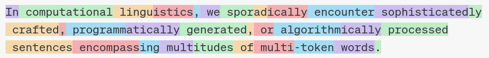
LLMs operate on tokens rather than words. For the purposes of this article we will use these two terms interchangeably, but it’s good to note the difference. Tokens are defined as frequently occurring sequences of characters, and often coincide roughly with words (and may even include the preceding space as well). A fun exercise is to play around with the GPT-4 tokenizer, which I used to generate the following example (color-coding reveals the underlying tokens):
 screenshot from https://platform.openai.com/tokenizer
The type of generative LLMs that most of us work with everyday are next-token-prediction machines. They have been trained (sometimes referred to as pre-training) on massive amounts of human generated text (books, newspapers, the internet, etc.) so that when fed a random snippet of sensible text, they are very good at predicting what the next word should be. This is sometimes referred to as Causal Language Modeling. When applied repeatedly, this autoregressive text generation process can generate very human-like sentences, paragraphs, articles, and so on.
Often we will want to take one of these foundation model LLMs, that have been pre-trained on massive amounts of text (like the Llama family of models from Meta), and continue the training a bit further, i.e. fine-tune them on a much smaller text dataset. This practice has roots in the broader field of transfer learning.
The goal here is to gently tweak, or customize, the LLM’s next-token-prediction behavior without majorly disrupting or corrupting the basic underlying “intelligence” that is manifested in the model weights — this leads to LLMs that retain most of the emergent abilities of the foundation model (like reading comprehension, the ability to converse, to reason…), but are now specialized for a specific task. For example, instruction-tuning means fine-tuning an LLM so that it can follow instructions.
There are many instruction-tuning datasets available on HuggingFace datasets hub, organized by task. Some datasets are for question answering, or text summarization. In the vast majority of cases, all these datasets share the same basic underlying schema, each data sample containing:
- a prompt, a.k.a. the instruction
- a completion, a.k.a. the response
In this setting, the goal of fine-tuning is to increase (ultimately maximize) the probability that the LLM will generate the completion when given the prompt as input. In other words, the response “completes” the prompt. We rarely, if ever, have any interest in altering the probability that the LLM will generate the prompt itself… which is just the input to the LLM.
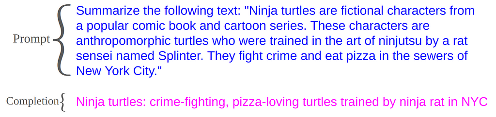 Text Summarization Example (image by the author)
Consider text summarization, for instance. A typical prompt might consist of an instruction to summarize a long news article together with the article itself, and the completion would be the requested summary (see the EdinburghNLP/xsum dataset on HuggingFace). The goal of fine-tuning a foundation LLM on this dataset would be to increase the likelihood that the LLM will generate the summary when given the instruction+article, not that the LLM will generate the article itself, or generate the second half of the article if shown the first half.
However, a popular approach that has emerged for fine-tuning LLMs on prompt-completion style datasets is to largely ignore the prompt-completion distinction, and fine-tune the model on the entire text sequence — basically just continuing the same process that was used to pre-train the foundation model, even though instruction tuning has a quite different goal from pre-training. This leads to teaching the LLM to generate the prompt as well as the completion.
I’m not entirely sure why this is the case, but most likely this habit was simply inherited from older, foundation model training protocols, where there was originally no such distinction. From what I can gather, the basic attitude seems to be: well, what’s the harm? Just fine-tune on the entire sequence, and the model will still learn to do what you want (to generate the completion given the prompt)… it will just learn some extra stuff too.
Prompt-Masking -vs- Prompt-Dampening
The most obvious solution would be to eliminate (or zero-mask) the prompt tokens out of the learning process. PyTorch allows for manually masking input tokens from training, through the ignore_index=-100 parameter of the CrossEntropyLoss function. Setting all the label ids corresponding to the prompt tokens to -100 forces CrossEntropyLoss to ignore these tokens in the loss computation, which results in training only on the completion tokens (in my opinion, this is a very poorly documented feature — I only stumbled upon it by accident — there’s a reference buried in here in the Llama documentation).
By itself, this is not really a solution to prompt-masking. It’s only a means for masking arbitrary tokens once those tokens have been located by some other means. Some of the prompt-masking references listed earlier employ this technique, while others explicitly create a binary-mask to accomplish the same thing. While useful, this solution is still a binary switch rather than the continuous dial that prompt-loss-weight allows.
However, this begs the question: if prompt-masking does improve instruction-tuning, what’s the point of having a non-zero prompt-loss-weight at all? Why would we want to merely dampen the influence of prompt tokens rather than eliminate it completely?
Recently a paper was posted on arxiv titled Instruction Fine-Tuning: Does Prompt Loss Matter? The authors suggest that a small amount of prompt learning may act as a regularizer during fine-tuning, preventing the model from over-fitting the completion text. They hypothesize:
…that [a non-zero] PLW provides a unique regularizing effect that cannot be easily replaced with other regularizers…Even the folks at OpenAI seem to acknowledge the benefits of using a small but non-zero prompt-loss-weight. Apparently they once exposed this very PLW parameter through their fine-tuning API, and there’s still some documentation about it online, in which it’s noted that:
a small amount of prompt learning helps preserve or enhance the model’s ability to understand inputs (from Best practices for fine-tuning GPT-3 to classify text)although they have since removed this parameter. According to the old docs, though, they used a default value of PLW=0.1 (10%), meaning prompt tokens get weighted 1/10ᵗʰ as much as completion tokens.
Generation Ratio
In the previously mentioned paper (Instruction Fine-Tuning: Does Prompt Loss Matter?) the authors introduce a useful quantity. Given an instruction dataset, they define the Generation Ratio, or Rg:
the generation ratio Rg is the ratio of completion length to prompt length. We then divide instruction data into two broad categories. Data with Rg<1 are short-completion data, and data with Rg >1 are long-completion data. When applied to an entire dataset, we take R̅g to be the mean completion-prompt ratio.For datasets with small R̅g values (i.e. the completion is shorter than the prompt) they found that PLW actually does matter (i.e. using the wrong PLW value can degrade performance). And if you think about it, many common instruction-tuning datasets have this property of having a shorter completion length than prompt length, almost by design (think: text summarization, information extraction)
As a fun exercise, I computed the R̅g values for several popular instruction datasets on HuggingFace (code here):
- 7.6 | Alpaca (general instruction)
- 6.0 | OpenHermes (general instruction)
- 3.6 | Python-18k (code instruction)
- 2.0 | Databricks-Dolly-15k (general instruction)
- 1.1 | OpenOrca (general instruction)
- 0.2 | SAMSum (text summarization)
- 0.1 | XSum (text summarization)
- 0.01 | RACE (QA/multiple choice)
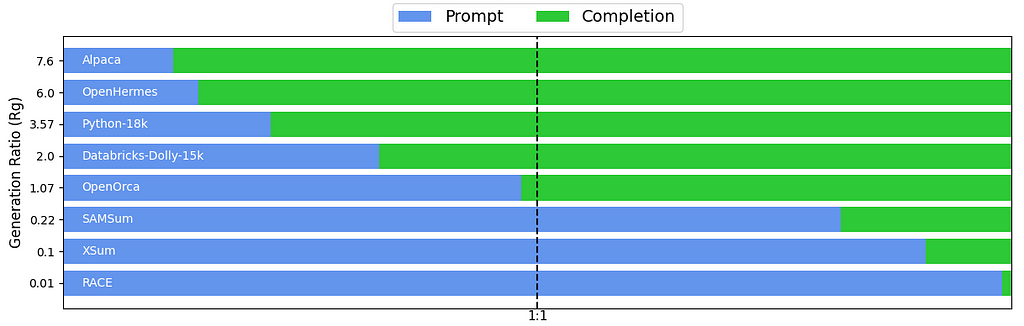 Mean Generation Ratio (R̅g) for some instruction datasets (image by the author)
When summarizing any set of values by its average, its good practice to look at the full distribution of values as a sanity check. The arithmetic mean can be misleading on data that is highly skewed or otherwise deviates from being roughly normally distributed. I plotted histograms showing the full Rg distribution for each dataset (top row). The bottom row shows the same histograms but with the x-axis log-scaled:
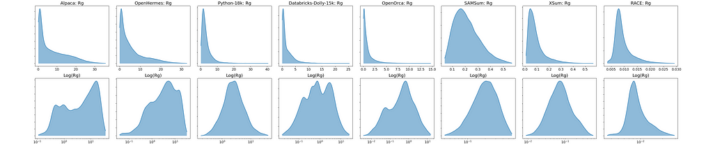 Linear and Log-scaled Rg Histograms (image by the author)
These plots suggest that when a dataset’s Rg distribution covers multiple orders of magnitude or has non-negligible representation in both the Rg>1 and Rg<1 regions (such as in the case with OpenOrca and other datasets with R̅g>1) the distribution can become highly skewed. As a result, the arithmetic mean may be disproportionately influenced by larger values, potentially misrepresenting the distribution’s central tendency. In such cases, computing the mean in log-space (then optionally transforming it back to the original scale) might provide a more meaningful summary statistic. In other words, it could make sense to use the geometric mean:
The RACE Reading Comprehension Dataset
Based on the above R̅g table, I decided the RACE ReAding Comprehension Dataset from Examinations (R̅g=0.01) would be a good candidate for investigation. Multiple choice QA seemed like an ideal test-bed for exploring the effects of prompt-masking, since the prompt is naturally very long relative to the completion. Regardless of prompt length, the completion is always 1 character long, namely A, B, C or D (if you ignore special tokens, delimiters, etc). My hunch was that if there are any effects from modulating prompt token weights, they would certainly be noticeable here.
As stated in the dataset card:
RACE is a large-scale reading comprehension dataset with more than 28,000 passages and nearly 100,000 questions. The dataset is collected from English examinations in China, which are designed for middle school and high school students. The dataset can be served as the training and test sets for machine comprehension.The QA schema is simple: the prompt presents a question, possibly some context (the article field), and then lists four options. The completion (answer) is always one of: A, B, C, D. This dataset viewer hosted on HuggingFace allows browsing the full set, but here’s a small example:
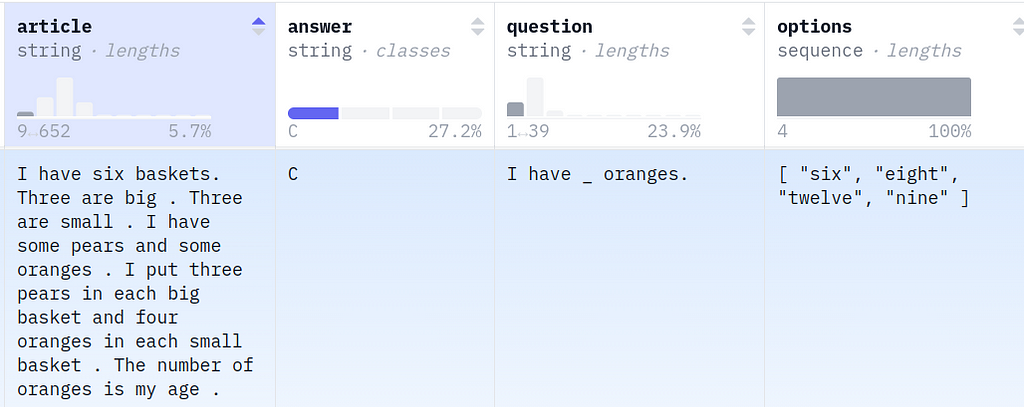 RACE example (screenshot from https://huggingface.co/datasets/ehovy/race/viewer/all/train)
Cross Entropy Loss
Before we jump into the full implementation of prompt-loss-weight, and try it out on the RACE data, we need a basic understanding of loss and where it comes from. Simply put, loss is a measure of how well our model (LLM) “fits” (explains, predicts) our data. During fine-tuning (and also pre-training), we “move” the model closer to the data by tweaking the network weights in such a way that decreases the loss. The chain rule (of calculus) gives us a precise algorithm for computing these tweaks, given the loss function and the network architecture.
The most common loss function in LLM fine-tuning is called Cross Entropy Loss (CEL). For this reason, most discussions of CEL are framed around the definition of cross-entropy, which comes from information theory. While it’s true that “cross-entropy” is right there in the name, a more intuitive understanding can be achieved when approaching CEL through the lens of maximum likelihood estimation (MLE). I’ll try to explain it from both angles.
We have already established that LLMs are wired for next token prediction. What this means is that the LLM is basically just a mathematical function that takes as input a sequence of tokens, and outputs a conditional probability distribution for the next token over the entire token vocabulary V. In other words, it outputs a vector of probability values of dimension |V| that sums to 1. (in set notation |S| denotes the number of elements, or cardinality, of a set S)
Let’s take a small toy example to illustrate how this works. Imagine that our training data contains the 4-token sequence: The bird flew away. Given the first 3 tokens (The bird flew), an LLM might output the following vector of probabilities for every possible 4ᵗʰ token — for the sake of simplicity, we’ll imagine that the 5 candidate tokens listed (in magenta) are the only possibilities (i.e. |V|=5). The function p(⋅) represents the conditional probabilities output by the LLM (notice they sum to 1):
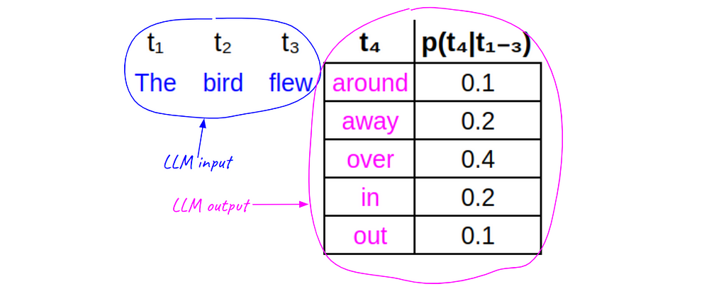 (image by the author)
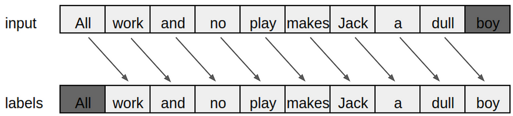
When training (or fine-tuning) an LLM on a token sequence, we step through the sequence token-by-token and compare the next-token-distribution generated by the LLM to the actual next token in the sequence, and from there we calculate the CEL for that token.
Notice here that the actual 4ᵗʰ token in the sequence (away) does not have the highest probability in the table. During training, we would like to tweak the weights slightly so as to increase the probability of away, while decreasing the others. The key is having the right loss function… it allows us to compute exactly how much to tweak each weight, for each token.
Once the loss is computed for each token, the final loss is computed as the average per-token-loss over all tokens. But first we must establish the formula for this per-token-loss.
Information Theory Interpretation
Continuing the toy problem, to compute CEL for the 4ᵗʰ token position, we compare the actual 4ᵗʰ token to the generated distribution p(⋅) over all 5 possible 4ᵗʰ tokens. In fact, we treat the actual 4ᵗʰ token as a distribution q(⋅) in its own right (albeit a degenerate one) that has a value of 1 for the token appearing in the data -away- and a value of 0 for all other possible 4ᵗʰ tokens (this is sometimes called one-hot encoding).
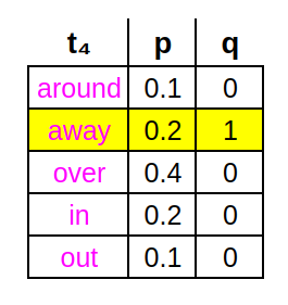 (image by the author)
The reason we contort the training data into this strange one-hot encoded probability representation q(⋅) is so we can apply the formula for cross-entropy, which is a measure of the divergence between two discrete probability distributions (BTW, not symmetric w.r.t. q,p):

where x indexes over all possible states (i.e. 5 tokens). This works out to:

So basically CEL is just using the q vector to select from the p vector the single value corresponding to the token that actually appears in the data -away- (i.e. multiplying it by 1), and throwing away all other values (i.e. multiplying by 0). So we are indexing over all possible states (tokens) only to select one and ignore the rest.
MLE Interpretation
When fine-tuning an LLM, we seek the LLM weights θ that maximize the probability of the training data given those weights, often called the likelihood of the weights ℒ(θ) = ℙ(D|θ). And so we require an expression for this quantity. Luckily, there’s an easy way to compute this from next token probabilities, which the LLM already gives us.
Starting with the other chain rule (of probability), we decompose the joint probability of a token sequence S into a product of conditional probabilities:
 Chain Rule (probability)
This decomposition establishes the connection between next-token-prediction and the joint probability of the full token sequence — the joint probability is just the product of all the conditionals.
Using i to index over the tokens of a token sequence S = (t₁,t₂,t₃,…, tᵢ ,…), we’ll use the following shorthand to denote the conditional probability output by an LLM for the iᵗʰ token in a sequence, given the LLM weights θ and the previous i-1 tokens:

It should be emphasized that pᵢ is not a vector here (i.e. a distribution over all possible next tokens) but represents only the probability computed for the actual iᵗʰ token, i.e. the yellow highlighted row in the above example.
If we take the logarithm of the joint probability of a sequence, a product becomes a sum (since log is monotonic, this doesn’t affect optimization):
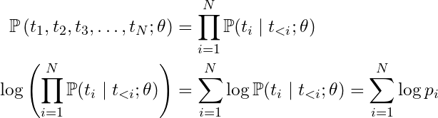
Now we can connect the final sum-of-logs expression (right here☝)️ to the formula for Average Cross Entropy Loss L over a token sequence:
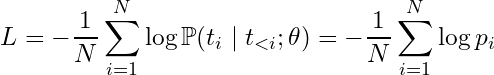
which is the causal language model objective function. Often the “Average” is dropped from the name, and it’s just called “Cross Entropy Loss,” but it’s good to remember that CEL is technically computed at the token level, and then averaged across tokens. From this final expression it should hopefully be clear that minimizing the CEL is equivalent to maximizing the probability of the token sequence, which is what MLE seeks.
One convenience resulting from the form of this expression is that it is very easy to modify if we want to compute the loss over any subset of the tokens. Recall that we may sometimes be interested in finding the LLM weights θ that maximize the probability of the completion given the prompt:
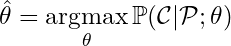
We could easily adjust the loss for this scenario by simply averaging only over the completion tokens. If we use “𝕀c” to denote the set of all completion token indices, then we can express completion loss as:
Since the loss for each token is already conditioned on all previous tokens in the sequence, this means that the prompt is automatically accounted for in the conditional, even if we average over completion tokens only.
Prompt Loss Weight
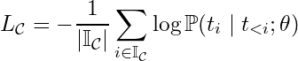
Now that we have established CEL as an average of per-token losses over a token sequence, we can define the weighted average version of CEL:
Depending how we set the weights wᵢ, we can use this formula to define multiple losses. For example, if we set all weights wᵢ =1 then we recover the standard, full sequence CEL from before. However, if we set wᵢ =1 only for completion tokens, and wᵢ = 0 for prompt tokens, then we get completion loss. And likewise, prompt loss is defined by setting wᵢ =1 only over prompt tokens, and wᵢ = 0 otherwise.
Since we rarely (if ever) want to down-weight the completion tokens, we fix the completion token weights at wᵢ =1, but for the prompt tokens we can define a continuous value on the [0:1] interval called prompt_loss_weight. This way we can tune how much to weight the prompt tokens during training, from wᵢ = 0 (completion loss) all the way to wᵢ =1 (standard full sequence loss). Or, we could even use wᵢ =0.1 to give the prompt tokens a small but non-zero weight.
Loss Implementation
Let’s take a look under the hood at how loss is normally computed in the HuggingFace transformers package. Since we’ll be fine-tuning the Llama-2–7b-chat-hf model in our experiments, we’ll look at LlamaForCausalLM, specifically at the forward pass, where loss is computed during training.
Recall that loss is a way of comparing each actual token to the LLM’s prediction for that token (given the preceding actual tokens) — and so the loss function needs access to these two data structures. In this case, loss is fed two tensors: logitsand labels. The labels tensor holds the actual tokens (token ids to be exact). Thelogits tensor holds the predicted next-token-probabilities, prior to softmax normalization (which forces them to sum to 1 — it turns out that it’s more efficient to leave these values in their raw, pre-normalized form).
The logits tensor is 3D, with shape [B,N,|V|], where B is batch size, N is sequence length (in tokens), and |V| is token vocabulary size. The 2D labels tensor just contains the token sequence itself, so it has shape [B,N]. Here is the key section of code where CEL is normally computed:
# Shift-by-1 so that tokens < n predict nshift_logits = logits[..., :-1, :].contiguous()
shift_labels = labels[..., 1:].contiguous()
# Flatten the tensors
shift_logits = shift_logits.view(-1, self.config.vocab_size)
shift_labels = shift_labels.view(-1)
# Enable model parallelism
shift_labels = shift_labels.to(shift_logits.device)
# Compute loss
loss_fct = CrossEntropyLoss()
loss = loss_fct(shift_logits, shift_labels)
For each position i along the 2nd dimension of logits, this tensor contains probabilities for predicting the next token (token i+1) given all the preceding tokens up through the iᵗʰ token. These probabilities need to be compared to the actual i+1ˢᵗ token in labels. This is why the shift-by-1 happens in the first several lines — to bring these two values into alignment for each token.
 (image by the author, inspired by: https://wandb.ai/capecape/alpaca_ft/reports/How-to-Fine-Tune-an-LLM-Part-2-Instruction-Tuning-Llama-2--Vmlldzo1NjY0MjE1)
What happens next is just that the first 2 dimensions are combined into 1 (flattened), and the tensors are passed to CrossEntropyLoss(), a PyTorch function, which outputs the final loss value.
Custom Loss Function
By default, CrossEntropyLoss() averages over all tokens to output a single scalar value. This final averaging (over all tokens) is called a reduction operation. But if we instantiate the loss with no reduction operation:
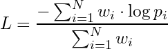
loss_fct = CrossEntropyLoss(reduction="none")then no averaging will be done, and the final loss would instead be a 1-D tensor (of length BxN) containing the losses for each token (the loss tensor would be 2D, shape [B,N], without the prior flattening step). That is how we get access to the per-token losses to compute our own weighted average.
During tokenization (see full code for details) we create two additional binary masks for each sequence, the prompt mask and the completion mask. A binary mask is just a vector of ones and zeros. The prompt mask marks all the prompt tokens with 1s (0s otherwise) and the completion mask does the opposite. Then we can use a simple linear combination of these two masks to get the weights wᵢ for the weighted average version of CEL, multiplying the prompt mask by PLW and adding to the completion mask:
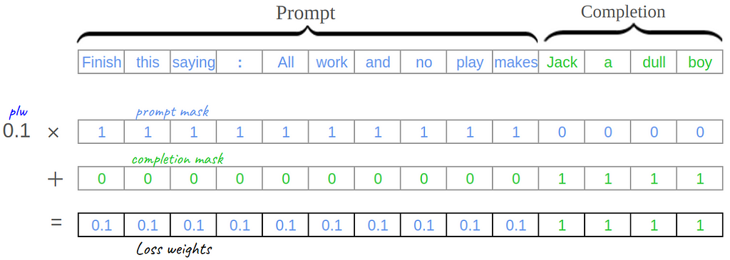 loss weights = prompt_loss_weight * prompt_mask + completion_mask (image by the author)
We subclass from HuggingFace Trainer to define a new trainer class called PLWTrainer. We’ll start by overriding just two functions:
- __init__(): constructor receives extra prompt_loss_weight parameter
- compute_loss(): computes weighted loss using prompt_loss_weight
def __init__(self, *args, prompt_loss_weight=1.0, **kwargs):
super().__init__(*args, **kwargs)
self.plw = prompt_loss_weight
def compute_loss(self, model, inputs, return_outputs=False):
# get outputs without computing loss (by not passing in labels)
outputs = model(input_ids=inputs["input_ids"],
attention_mask=inputs["attention_mask"])
logits = outputs.get("logits")
labels = inputs.pop("labels")
# compute per-token weights
weights = self.plw * inputs["prompt_mask"] + inputs["completion_mask"]
# Shift-by-1 so that tokens < n predict n
shift_logits = logits[..., :-1, :].contiguous()
shift_labels = labels[..., 1:].contiguous()
shift_weights = weights[..., 1:].contiguous()
# Enable model parallelism
shift_labels = shift_labels.to(shift_logits.device)
shift_weights = shift_weights.to(shift_logits.device)
# Compute per-token losses
loss_fct = CrossEntropyLoss(reduction="none")
token_losses = loss_fct(shift_logits.view(-1, shift_logits.size(-1)),
shift_labels.view(-1))
# Compute weighted average of losses
loss = token_losses @ shift_weights.view(-1) / shift_weights.sum()
return (loss, outputs) if return_outputs else loss
If no explicit value is passed to the constructor for prompt_loss_weight, the default value (prompt_loss_weight=1) means we revert to the inherited behavior of the original Trainer (i.e. minimizing full sequence loss). However, if we pass in other values for prompt_loss_weight, we get back a whole spectrum of different loss functions.
We’re almost ready to try our new loss function! But first we need to make sure we’re equipped to observe and understand what effect it’s having on the fine-tuning process, if any…
Validation Metrics
Tracking Prompt & Completion Losses Separately
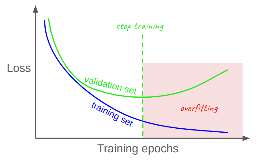
During fine-tuning, it is common practice to track model performance on a hold-out set in order to decide when to end training. The hold-out set, also called the validation set, is just a random subset of data that is literally “held-out” from the training data to ensure it isn’t learned/memorized by the model. The model’s performance on this set is seen as a proxy/estimate for how the model would perform in the real-world on new, unseen data. This is where the classic “training vs. validation curve” taught in most intro ML courses comes from:
 (image by the author)
The lesson here is that the minimum point of the green (validation) curve represents the optimal number of training steps, past which the model starts to overfit, or memorize, the training data, rather than continuing to learn generalizable patterns from the data. It’s impossible to know the true optimal stopping point, but tracking validation set metrics allows us to estimate it fairly well. Still, there is a trade-off: a larger validation set leads to a better estimate, but also leads to a smaller training set, so we don’t want to hold-out too many samples. 5%–15% is a good rule-of-thumb.
Typically, when fine-tuning LLMs, the objective loss function being minimized on the training set also becomes the default metric used to track the validation set performance, and thus determine the optimal stopping point. The discussion usually centers around two options:
- Minimize full sequence loss on train set — and track it on validation set
- Minimize completion loss on train set — and track it on validation set
But — we’re free to track any metric (or metrics) we want on the validation set, not just the loss being used as the training objective . This leads to the original idea that inspired this article — I wanted to try a third option:

However, after re-framing my approach around PLW, this evolved into:

To do this, we first need to write a custom metric to decompose validation full sequence loss into prompt loss and completion loss, which we do in the next section. We’ll use the same tricks we used in our custom loss function.
Digression: you may notice in the LLM community that practitioners sometimes sidestep the stopping criteria issue altogether by following a simple rule like always fine-tune for one epoch only, or something similar. Sometimes this makes sense, like when fine-tuning a model to produce text that’s more subjective, like emails, or poetry, or jokes. But when the fine-tuning dataset is aimed more at correctness, like writing code, solving math problems, or multiple choice QA (an example we will see below), then it definitely does make sense to monitor the validation loss, and/or other validation metrics. So it’s important to make sure we do it carefully.
However, this is not to say that the correctness of a token sequence is a simple linear function of individual token correctness. The semantic meaning of a token sequence can be a complex, highly non-linear function of the meaning of the individual tokens. That’s why it’s easy to construct many examples where one tiny change at the token level can dramatically alter the meaning of the whole — just insert “not” at the right place to completely invert the meaning of a sentence!.
Even so, in many cases the average per-token loss can still serve as a good indicator for the overall quality of LLM predictions during training/fine-tuning. This is because the standard practice of teacher forcing ensures that each token prediction is conditioned on the “correct” (i.e. ground truth) previous tokens from the train/validation data, as opposed to conditioning each token prediction on the model’s own previous token predictions (which is what happens during inference/text-generation).
But no single metric is perfect, which is why it’s always important to use multiple evaluation methods, including task-specific metrics, along with human evaluation.
Defining Custom Metrics
A common method for defining custom validation metrics, when using HuggingFace Trainer, is to override Trainer’s default compute_metrics() function that is periodically run on the validation set during training. However, this function does not, by default, receive enough information for computing prompt loss or completion loss.
Specifically, for each validation set sequence compute_metrics() receives the predicted tokens and the actual tokens. This is only suitable for computing certain metrics like token accuracy, but not for computing loss. Luckily, we can tinker with the data that’s passed into compute_metrics() by overriding another function, preprocess_logits_for_metrics().
To compute loss, we need access to the actual probability distributions contained in the logits. Recall that an LLM for next token prediction will, at each point along a token sequence, produce a probability distribution over all possible tokens in the vocabulary (|V|=32000) for the next token. This distribution is stored in logits, which has shape [B,N,|V|].
By default, preprocess_logits_for_metrics() will take the argmax (along the last dimension, the |V| dimension) of this logits tensor, and pass these token indices along to compute_metrics()
# from preprocess_logits_for_metricspredictions = logits.argmax(-1)[..., :-1]
These predictions represent the tokens the LLM would have predicted for every token position in every validation sequence, given the preceding tokens (final token prediction is chopped off because there’s no ground truth to compare it to). But as we have seen, to compute per-token losses we actually don’t need to know the highest probability tokens (predictions returned by argmax) — we need to know the probability the LLM assigned to the actual tokens in each validation sequence, given the preceding tokens.
One solution would just be to pass the entire logits tensor along to compute_metrics(), and then compute losses in there, along with any other metrics, like accuracy. There is a serious problem with that approach, though: the way Trainer is set up, the preprocess_logits_for_metrics() function is run (in batches) on the GPU(s), but compute_metrics() is run on the CPU (on the entire validation set as a whole — i.e. all batches recombined). And, the reason preprocess_logits_for_metrics() is run on GPU is that the logits tensor can get extremely large.
Just to give you an idea how large, in my experiments, I have been using a batch size (B) of 8, and sequence length (N) of 2048, which leads to a tensor containing B x N x |V| = 8 x 2048 x 32000 ≈ 4.2 billion values (per-GPU)!
The GPU can handle this giant tensor, but the CPU would explode if we tried to pass it along. We must perform some sort of reduction first, inside preprocess_logits_for_metrics(), to eliminate this giant 3rd dimension.
There’s no single right way to do this. One option would be to select from logits the probability generated for every actual (true) token, and pass these along to compute_metrics(), then compute the losses there on the CPU. That would certainly work. However, a better idea would be to use the full processing power of the GPU(s) to do a bit more computation inside preprocess_logits_for_metrics() before handing things off to the CPU side.
Recall that cross entropy loss over a token sequence is just the average per-token loss over the whole token sequence. So we can use preprocess_logits_for_metrics() to compute a tensor containing all the per-token losses, and pass this tensor to compute_metrics() to do the averaging later on.
One minor complication is that preprocess_logits_for_metrics() is set up to pass a single value on to compute_metrics(). However, we need to pass along two separate tensors. Since we’re interested in tracking multiple metrics on the validation set (prompt loss and completion loss, as well as completion token accuracy) — we require two tensors: predictions for completion accuracy, and per-token-losses for both losses. Luckily, the single value passed from preprocess_logits_for_metrics() to compute_metrics() can be a either a single tensor or tuple of tensors.
Specifically, compute_metrics() receives a single argument data which is an instance of the utility class transformers.EvalPrediction. The value returned by preprocess_logits_for_metrics() is assigned to the .predictions field of EvalPrediction (after batches are gathered into a single tensor, and converted to numpy arrays). The spec for .predictions indicates that it can hold either a single array or a tuple of arrays (predictions: Union[np.ndarray, Tuple[np.ndarray]]) so we are good to go.
# uses PyTorch tensors (on GPU)def preprocess_logits_for_metrics(logits, labels):
# get predictions
token_preds = logits.argmax(-1)[..., :-1]
# compute per-token losses
loss_fct = CrossEntropyLoss(reduction="none")
shift_logits = logits[..., :-1, :].contiguous()
shift_labels = labels[..., 1:].contiguous()
token_losses = loss_fct(shift_logits.transpose(1, 2), shift_labels)
# pass predictions and losses to compute_metrics()
predictions = (token_preds, token_losses)
return predictions
Now we can define compute_metrics()…
# uses numpy arrays (on CPU)def compute_metrics(data):
# data.predictions contains the tuple (token_preds, token_losses)
# from preprocess_logits_for_metrics()
token_preds, token_losses = data.predictions
# shift labels and masks
labels = data.label_ids[..., 1:]
shift_prompt_mask = prompt_mask[..., 1:]
shift_comp_mask = completion_mask[..., 1:]
# average both losses (prompt and completion) over their respective tokens
prompt_loss = token_losses.reshape(-1) @ shift_prompt_mask.reshape(-1) / shift_prompt_mask.sum()
completion_loss = token_losses.reshape(-1) @ shift_comp_mask.reshape(-1) / shift_comp_mask.sum()
# compute response token accuracy
nz = np.nonzero(shift_comp_mask)
idx = np.where(np.isin(labels[nz], ABCD_token_ids))
accuracy = np.mean(preds[nz][idx] == labels[nz][idx])
return {
'comp_loss': completion_loss,
'prompt_loss': prompt_loss,
'acc': accuracy,
}
This should all look familiar because we are using the same ideas we used to define our custom loss function. Again, we rely on prompt_mask and completion_mask to select the proper token subsets for computing each loss. If you are wondering where prompt_mask and completion_mask are defined, it happens outside the function scope but they are made available using a function closure, a method often employed in “function factories” (see full script for details).
The completion token accuracy is computed only on the actual multiple choice answer token (i.e. A,B,C,D), whereas completion loss includes other special tokens used in the chat template (i.e. spaces, bos_token, eos_token, etc). The referenced ABCD_token_ids allows us to isolate the answer tokens and ignore other tokens.
Experiments
Finally, let’s do some fine-tuning runs while varying PLW…
Full Sequence Training: PLW=1
Implementation details: I use Llama-2–7b-chat-hf as the base model, and fine-tune it on a subset of the RACE reading comprehension dataset using the LoRA (Low-Rank Adaptation) method via the HuggingFace PEFT (Parameter Efficient Fine-Tuning) library. I was able to speed up fine-tuning considerably with multi-GPU training using Microsoft’s DeepSpeed library. Again, see full code for all the details.
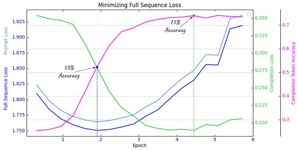
This first plot below tracks the evolution of all validation set metrics when minimizing the standard, full sequence loss on the training set. Each curve has it’s own y-axis labels (color-coded) since they are all on different scales (except prompt and full sequence loss, which use the same scale, on left). You can see that response accuracy tracks very closely with completion loss, but opposite in direction, as should be expected. I’ve drawn dashed blue and green lines through the minima of completion loss and full sequence loss, to show where each intersects with accuracy.
 RACE Validation Set Metrics (image made with Matplotlib by the author)
The main thing to observe is how the minima of prompt loss and completion loss are extremely out of sync — since prompt loss dominates full sequence loss (remember R̅g = 0.01) the full sequence loss is basically just prompt loss shifted down slightly, and they share the same arg-min.
This means that if you blindly follow popular practice and use the minimum of validation full sequence loss as the stopping criterion — just shy of epoch 2— where completion loss is still very high — the fine-tuned model would only have 53% accuracy!
But, by merely tracking the completion loss separately (as opposed to direct minimization by using PLW=0 in our custom loss function, which we’ll do next) you would continue fine-tuning to 4.5 epochs, where completion loss reaches its minimum, and increase accuracy to 75% !
Completion Only Training: PLW=0
Now, we’ll swing to the opposite end of the spectrum and completely mask out the prompt tokens. All we have to do is initialize the PLWTrainer with prompt_loss_weight=0. Here are those results plotted:
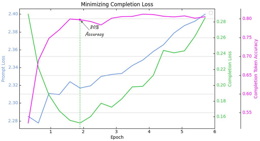 RACE Validation Set Metrics (image made with Matplotlib by the author)
Two important things have changed:
- fine-tuning converges much faster to the minimum completion loss -and optimal accuracy - taking < 2 epochs (instead of 4.5 epochs)
- the optimal accuracy is higher as well — jumping from 75% to 80%
Another interesting thing to notice is that the prompt loss doesn’t go down at all, like in the previous plot, but just kind of floats around, even drifting slightly higher (pay close attention to the prompt loss y-axis scale — on the left). In other words, there is absolutely no learning over the prompt tokens, and eliminating them from fine-tuning has improved both the convergence speed and the maximum accuracy achieved. Seems like win/win!
Exploring The Full PLW Spectrum
Recall that if we use any fractional value 0 < PLW < 1 then the influence of prompt tokens on the total loss is dampened but not eliminated. Below I have plotted the validation set completion loss and the QA accuracy at six different PLW values: [1, 0.5, 0.2, 0.1, 0.01, 0]
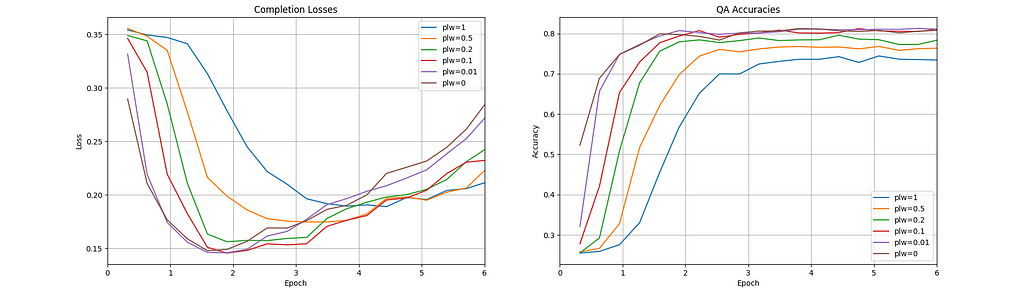 RACE Validation Set Metrics (image made with Matplotlib by the author)
What is most striking is how much faster the completion loss converges to the minimum for the three lowest PLW values [0,0.01,0.1]. The fastest convergence seems to happen at PLW=0, but only by a small amount compared to the next two smallest values. Looking at the accuracies, it appears that any of the three lowest PLW values will achieve the optimal accuracy (~80%) by around epoch 2.
It’s also interesting to compare the convergence behavior of each completion loss curve to its corresponding accuracy curve. After reaching their minima, all six completion loss curves begin to slowly increase, while all accuracy curves level off without decreasing… How can we explain this?
Digression: Loss or Token Accuracy — Which to track?
Recall that next token prediction is done by selecting the token with the highest probability given the previous tokens. The formula for token accuracy only considers if the token is correct or not, whereas the formula for Cross Entropy Loss actually takes into account the values of these probabilities. So what could be happening to explain the difference between these two graphs?
Well, since the token accuracies are holding steady, this implies that the tokens having the highest probabilities (the argmax tokens) are remaining fairly constant, but those max values must be steadily declining — in other words, the model is becoming less confident about its (mostly correct) token predictions. This could be viewed as just mild case of overfitting, where the max values are affected, but not enough to affect the argmax values.
This example illustrates why some say that tracking token accuracy is better than tracking validation loss. Personally, I think its silly to argue about which one is better than the other, because you don’t have to choose… track both of them! Both are valuable indicators. Token accuracy may be ultimately what you care about maximizing (in many cases, anyway…). But I would also like to know if and when a model is becoming less confident in its (mostly) correct predictions (like we see above) so I would track completion loss as well.
Better yet, the optimal strategy (in my opinion) would be to also track the model’s performance on a benchmark, or a suite of benchmarks, to get a fuller picture of how it’s evolving throughout the fine-tuning process. It could be the case that your LLM is getting better and better in terms of pure token accuracy on the validation set, but at the same time its responses are becoming more repetitive and robotic sounding, because the validation set is not diverse enough (I have actually seen this happen, in my day job). It’s always important to keep in mind what the true, ultimate goal is… and in almost all cases, token accuracy on the validation set is a mediocre proxy at best for your true goal.
Conclusion
Our exploration into the effects of varying prompt-loss-weight on LLM instruction-tuning has highlighted several important concepts:
- Decoupling training objective from validation metrics: Even without changing how prompt tokens are weighted inside the training objective function, we saw that we could improve our results just by tracking the right validation metric (i.e. completion loss, or accuracy).
- PLW can effect model performance: By decreasing PLW, we saw our fine-tuned model performance improve. Surprisingly, full prompt-masking was not required to achieve maximal improvement, since decreasing PLW below 0.1 seemed to have no additional effect. Whether or not this behavior translates to other datasets must be evaluated on a case by case basis.
- PLW can effect convergence speed: Again, by decreasing PLW, we saw our fine-tuned model converge much faster to its optimum. This effect may be largely independent of the effect on model performance — i.e. depending on the dataset, either effect may appear without the other.
- Dataset-Specific Optimization: Depending on the specific dataset and task, it’s very likely that the optimal PLW will vary widely. It’s even possible that in many cases it could have no effect at all. The dramatic improvements seen with the RACE dataset may not generalize to all fine-tuning scenarios, highlighting the need for experimentation.
Future research directions could include:
- Exploring the effects of PLW on a wider range of datasets beyond instruction datasets, such as those with larger generation ratios, or with longer chat dialogues
- Developing adaptive PLW strategies that adjust dynamically during the fine-tuning process
- Examining the impact of PLW on other aspects of model performance, such as generalization and robustness
I hope you’ve found this slightly useful. I’m always open to feedback and corrections! The images in this post are mine, unless otherwise noted.
Resources
- All codes related to this tutorial can be accessed here.
To Mask or Not to Mask: The Effect of Prompt Tokens on Instruction Tuning was originally published in Towards Data Science on Medium, where people are continuing the conversation by highlighting and responding to this story.


 English (US)